Mazes 3.: Border mazes -- Part 1.

Introduction

Administrative map-like structures will be generated in this blog post utilising a handful of simple graph theoretic algorithms. The first installment of this series saw the definition of mazes and basic procedures to create them. Images were turned in to mazes in the second post. A country is divided in to smaller non-overlapping and adjoining areas such as counties (England), regions (France), states (USA) which are, in turn partitioned in to even smaller units. E.g. parishes, arondissements, counties at various levels. Three German divisions are shown in Figure 1. The idea naturally arises that removing sections of the borders between administrative areas at the same level a maze can be created.

jpg

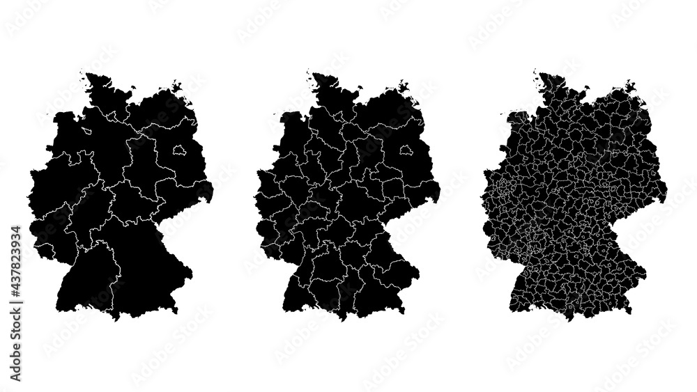
Figure 1. The first (left panel), second (right panel) and third (right panel) level administrative division of Germany. The walls are marked up in white.

Notes

The raw notebook can be found here. The scripts are deposited in this repository.

Problem statement

Unfortunately, the publicly available and free administratie region databases [1, 2] contain borders that are not always adjoining or overapping. The closest to this dual criterion comes is the magnum opus of the French cartographers. Still, roughly only the quarter of the neighbouring border segments is overlapping.

We therefore set out to create our own administrative region maps where the all of the borders comply with the two requirements.

Procedure

The idea is simple. A random pointset is created which then triangulated. Some triangles are merged to form the quasi areas. The outlines of these are then read off.

Estimation of the number of triangles

Let us require $N$ subdivisions each having a border composed of $M$ segments. Furthermore, let us assume that each area is approximated by a square. Then the number of triangles, $m$ in an area is

\[m \approx \left[ \frac{M}{4} \right ]^{2}\]

The total number of triangles is $N \cdot m$. Let $s$ be the minimum side length of a triangle, so that one will take up a space roughly $s^{2} / 2$ pixels. Overall

\[P = N \cdot \frac{M^{2}}{16} \cdot \frac{s^{2}}{2} = N \cdot \frac{M^{2}s^{2}}{32}\]

pixels must be in the canvas. Again, if the canvas is a square then its side length is

\[l = \sqrt{\frac{N \cdot M^{2}s^{2}}{32}} = \sqrt{\frac{N}{2}} \cdot \frac{M \cdot s}{4}\]

Let us say 1000 countries of borders composed of 100 of the tiniest possible triangle size of 3 would require

\[l = \sqrt{\frac{1000}{2}} \cdot \frac{100 \cdot 3}{4} \approx 1700\]

long square canvas.

Pointsets

Random points on a grid

A function, sample_drawing_points_2d was written in Part 1 to scatter the plane with random points and is used again. The canvas size is set rather large for we wish to have fine details of the borders.

Trimming

The Delaunay triangulation yields sliver triangle along the convex hull of the pointset. They may lead to borders with long sharp edges. There are three solutions to remove them

add Steiner points
create and alpha shape
trim the rectangular pointset to a shape whose convex hull is likely to be composed of short segments.

We choose the last option for its simplicity. The shape is an ellipse. Function trim_in_ellipse removes points outside of an ellipse. A slighly smaller map with fewer subdivisions is constructed for demonstration purposes. The points are scattered on Figure 2.

height_canvas = 700
width_canvas = 1000
width_border = 20
shift = div(width_border, 2)

n_points = 300000
r_x = div((height_canvas - width_border), 2)
r_y = div((width_canvas - width_border), 2)

xy = Maze.sample_drawing_points_2d(n_points, height_canvas, width_canvas, 1, 1)
xy = Maze.trim_in_ellipse(xy, r_x, r_y, r_x, r_y)

png

Figure 2. The points over which the regions will be defined.

Triangulation

The Delaunay graph is constructed by invoking the TriGraph function developed in the first post. The triangulation is the subject of Figure 3. The area of triangles will form the mass of the regions whereas some of their sides will mark the borders.

graph = Maze.TriGraph{Int}(xy)

png

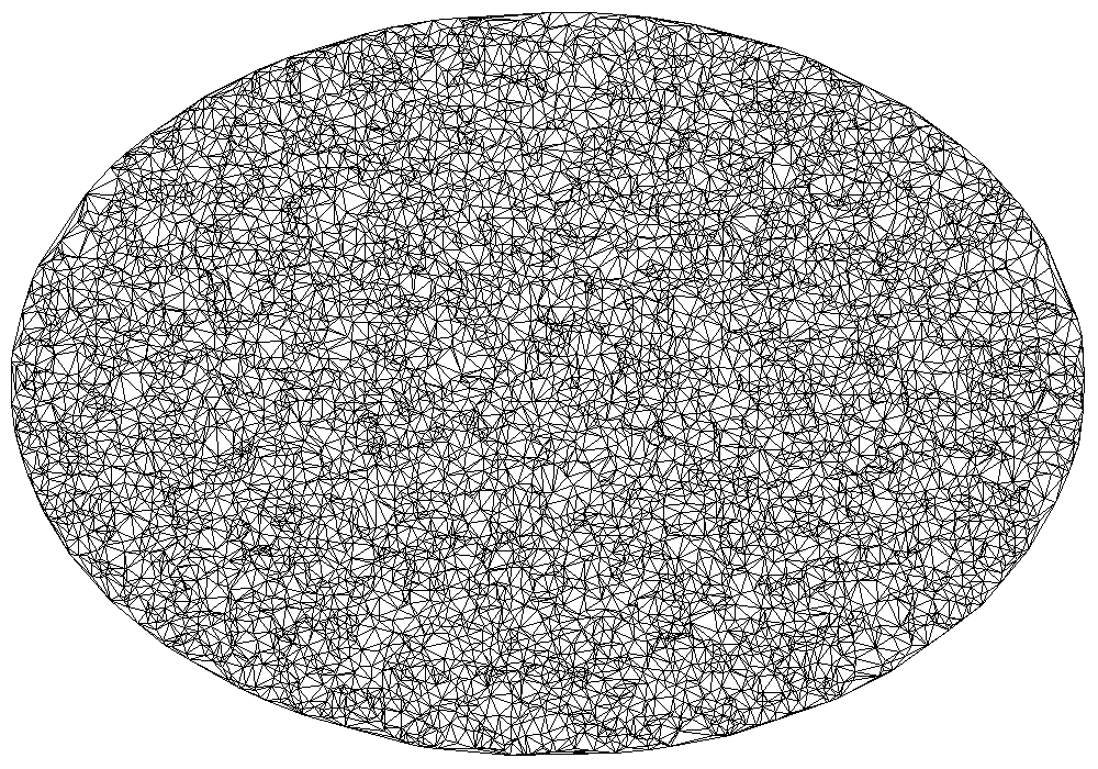
Figure 3. The triangulation.

Merging regions

A single pass algorith is defined which merges adjoining triangles.

Initialisation

A number, $N$ of triangles are selected as the seed of the regions. The initialisation step of the $k$-means++ algorithm chooses points which are suitably far from each other on average.

Merging

Let $G=(\mathcal{V}, \mathcal{E})$ a directed multigraph:

\[\begin{eqnarray} ! \mathcal{V} & \neq & \emptyset \\ ! \emptyset & \neq & \mathcal{E} \subset \mathcal{V} \times \mathcal{V} \\ \forall (s, t) & \in & \mathcal{E}: s \neq t \quad \text{(no self cycles)} \\ \forall (s, t) & \in & \mathcal{E} \leftrightarrow (t, s) \in \mathcal{E} \quad \text{(symmetric)} \end{eqnarray}\]

We seek a decomposition of the graph where the components are disjoint and connected. $\begin{eqnarray} \bigcup\limits_{i=1}^{N} \mathcal{W}_{i} & = & \mathcal{V} \quad \text{(all vertices included)} \\ \forall i, j & \in & [1, N], i \neq j: \mathcal{W}_{i}\cap \mathcal{W}_{j} = \emptyset \quad \text{(disjoint sets)} \\ \forall i, \forall s, t & \in & \mathcal{W}_{i}: \text{Connected}(s, t) \end{eqnarray}$

Let us start with the set of starting vertices, $\mathcal{S}$.

while there are vertices in the graph
choose a vertex
select a second vertex from the neighbours
propagate label
remove the second vertex from the neighbours of the first vertex
if the first vertex has no out-edges, remove it from the graph
remove all in-edges pointing to the second vertex from the neigbours of the second vertex
if the second vertex has no out-edges remove it from the graph

The crucial steps are 5. through 7. If a vertex has been labeled there is no point visiting it again. Only unlabeled vertices have in edges which are out-edges from other (labeled or unlabeled) vertices. The algorithm terminates because out-edges of unlabeled vertices can only be removed from labeled ones.

There is a catch, however, when trying to implement the algorithm sketched out above. When the in-edge of an labeled vertex, $t$ is removed from the neighbours of an unlabeled vertex $r$ then edge from $t$ to $r$ remains. If $r$ becomes labeled from $u \neq t$ the edge from $t$ must be deleted. However, $r$ has no reference to $t$ anymore thus there will be an edge from $t$ pointing to the now labeled $r$ which is not allowed.

It is possible to introduce a check on the neighbours of $t$ when it becomes the current vertex. This may lead to threshing – e.g. cycles spent on not propagating the labels if the only remaining neighbour of $t$ is $r$.

It is more efficient to create a copy of the original graph in which edges and vertices are deleted whilst using the original one for lookup on which approach the algorithm and function decompose_graph are based.

\[\begin{eqnarray} & \, &\text{Algorithm } \texttt{DecomposeGraph} \\ % & \,& \textbf{Inputs: } G=(\mathcal{V}, \mathcal{E}), & \quad \text{(graph)} \\ % & \,& \mathcal{S} \subset \mathcal{V} & \quad \text{(seeds)} \\ % & \,& \textbf{Output: } \mathcal{L} \in \mathcal{V} \times [1,N] & \quad \text{(labels)} \\ % & 1. & \quad \mathcal{L} \leftarrow \emptyset & \quad \text{(labels)} \\ % & 1. & \quad \mathcal{A} \leftarrow \mathcal{G} & \quad \text{(create an active graph)} \\ % & 1. & \quad \mathcal{Q} \leftarrow \emptyset & \quad \text{(active vertices)} \\ % & 1 .& \quad \textbf{for } i \in 1, |\mathcal{S}| \\ % & 1.& \quad \quad \mathcal{L} \leftarrow \mathcal{L} \cup (s_{i}, i) & \quad \text{(seed labels)} \\ % & 1. & \quad \quad \textbf{for } \forall t \in N_{out}(\mathcal{G}, s) & \quad \text{(use the original grap for lookup)} \\ % & 1. & \quad \quad \quad \mathcal{N}_{out}(\mathcal{A},t) \leftarrow \mathcal{N}_{out}(\mathcal{A},t) \setminus \{ s \} & \quad \text{(manipulate the active graph only)} & \\ % & 1. & \quad \quad \textbf{end for} & \\ % & 1. & \quad \textbf{end for} & \\ % & 1. & \quad \textbf{for } \forall s \in \mathcal{S} & \\ % & 1. & \quad \quad \textbf{if } |\mathcal{N}_{out}(\mathcal{A}, s)| = 0 & \\ % & 1. & \quad \quad \quad \mathcal{A} \leftarrow \mathcal{A} \setminus \{s\} & \quad \text{(remove from graph with edges)} \\ % & 1. & \quad \quad \textbf{else} &\\ % & 1. & \quad \quad \quad \mathcal{Q} \leftarrow \{ s \} & \quad \text{(add to the active set)} \\ % & 1. & \quad \quad \textbf{end if} & \\ % & 1. & \quad \textbf{end for} & \\ % & 1. & \quad \textbf{while} |\mathcal{A}| \neq 0 & \\ % & 1. & \quad \quad s \leftarrow \texttt{SelectVertex}(\mathcal{Q}) & \\ % & 1. & \quad \quad t \leftarrow \texttt{SelectNeighbour}(\mathcal{A}, s) & \quad \text{(only consider neigbours in the active graph)} \\ % & 1. & \quad \quad \mathcal{L} \leftarrow \mathcal{L} \cup (t, \mathcal{L}(s)) & \quad \text{(propagate label)} \\ % & 1. & \quad \quad \textbf{for } \forall r \in \mathcal{N}_{out}(\mathcal{A}, t) & \quad \text{(lookup all neigbours)} \\ % & 1. & \quad \quad \quad \textbf{if } r \in \mathcal{A} & \\ % & 1. & \quad \quad \quad \quad \mathcal{N}_{out}(\mathcal{A, r}) \leftarrow \mathcal{N}_{out}(\mathcal{A, r}) \setminus \{ t \} & \quad \text{(remove from neigbours)} \\ % & 1. & \quad \quad \quad \quad \textbf{if } |\mathcal{N}_{out}(\mathcal{A, r})| = 0 \land r \in \mathcal{L} & \quad \text{(vertex has no neighbours and labeled)} \\ % & 1. & \quad \quad \quad \quad \quad \mathcal{A} \leftarrow \mathcal{A} \setminus \{ r \} & \quad \text{(remve from the active graph)}\\ % & 1. & \quad \quad \quad \quad \quad \mathcal{Q} \leftarrow \mathcal{Q} \setminus \{ r \} & \quad \text{(remove from the active set)} \\ % & 1. & \quad \quad \quad \quad \textbf{end if} & \\ % & 1. & \quad \quad \quad \textbf{end if} & \\ % & 1. & \quad \quad \textbf{end for} & \\ % & 1. & \quad \quad \textbf{if } |\mathcal{N}_{out}(\mathcal{A}, t)| = 0 & \\ % & 1. & \quad \quad \quad \mathcal{A} \leftarrow \mathcal{A} \setminus \{ t \} & \quad \text{(remve from the active graph)}\\ % & 1. & \quad \quad \quad \mathcal{Q} \leftarrow \mathcal{Q} \setminus \{ t \} & \quad \text{(remove from the active set)} \\ % & 1. & \quad \quad \textbf{else} & \\ % & 1. & \quad \quad \quad \mathcal{Q} \leftarrow \mathcal{Q} \cup \{ t \} & \quad \text{(ensure it is in the active set)} \\ % & 1. & \quad \quad \textbf{end if} & \\ % & 1. & \quad \textbf{end while} & \\ % & 1. & \quad \textbf{return } \mathcal{L} & \\ % & 1. & \textbf{end function} & \\ % \end{eqnarray}\]

The $\texttt{SelectVertex}$ function chooses a vertex in the graph which has been labeled. Depending on the selection rules, the relative sizes of the regions can be controlled.

In the simplest case, it only takes a the active set as its sole argument and chooses a vertex with uniform probability. This will result in a rich-gets-richer scheme where those regions wich have more active vertices have a higher chance of being grown. Alternatively, the labels can be sampled uniformly which would lead to a partition of more balanced regions sizes.

The $\texttt{SelectNeighbour}$ simply picks a neighbour of a vertex. The partitioned graph is plotted in Figure 4.

n_seed = 200
seeds = Maze.init_seeds(xy, n_seed)
labels = Maze.decompose_graph(graph, seeds)

png

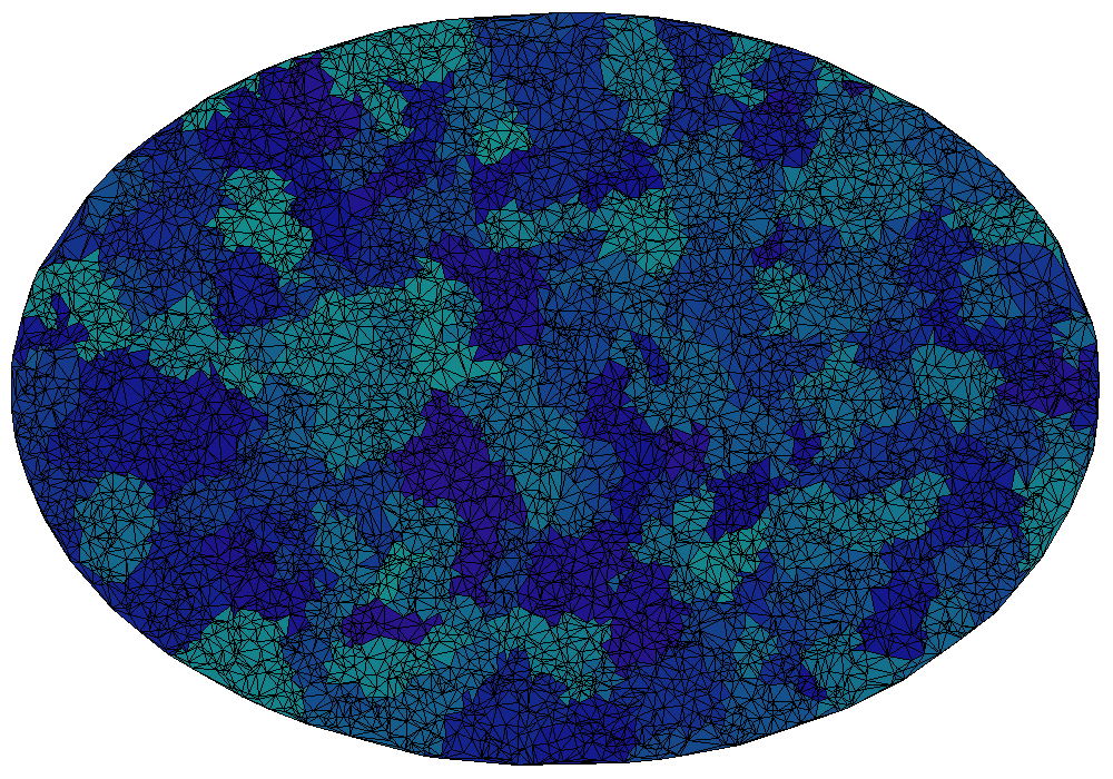
Figure 4. The decomposed graph.

Extraction of borders

By now there is a decomposed graph which consist of the graph itself and a map of vertex labels. The aim is to obtain those edges which either

are on the border of the entire area
are shared by two subdivisions

External border

The external border of a region – if exists – is composed of triangle sides whose have at least a single side the face the outer area when plotted. This provides a straignforward way to mark up the outer facing sides.

The mapping_edge_side field of the TrigGraph structure maps the edges (pairs of adjacent triangles) to the side by which they are connected. It is a bijection hence it can be inverted. This side-to-edge mapping is utilised to identify the external borner segments.

loop over all vertices
if a vertex has less than three neigbours
1. look up its sides where a side is a tuple of the indices of the points
2. look up whether this side is in the side–edge mapping
3. if not
  1. save it as an external border segment

Function extract_borders_external performs the above steps and returns a dictionary keyed by the labels under which the external border segments are collected.

Internal border

A internal border is the collection of sides that are between two regions. That is the two triangles of an internal border edge have different labels. This observation allows for marking up the segments using the edge–side mapping.

loop over all edge–side pairs in the mapping
look up vertex labels of the edges
if the vertex labels are not identical
1. save the side as an internal border segment.

Function extract_borders_internal groups the internal border segments by labels. The extract_borders thin wrapper collects and groups both types of border per label.

border_segments = Maze.extract_border_segments(graph, labels)

Linking or border segments

The border segments have now been collected. They only need to arranged in a chain of subsequent points. The naive approach would require $\mathcal{O}(N^{2})$ comparisons where $N$ is the number of segments. The task is solvable in $\mathcal{O}(N)$ time using hashing. Firstly, a graph is constructed where a vertex is a point index. An edge is added between two points if they appear in the same segment. A depth first search will yield the ordered point indices afterwards. chain_border_segments performs these two steps. Figures 5. and 6. display the borders with and without the regions highlighted.

borders = Array{Array{Int, 2}, 1}()
for (label, segments) in border_segments
    indices = Maze.chain_border_segments(segments)
    border = xy[:, indices] .+ [shift, shift]
    push!(borders, border)
end

png

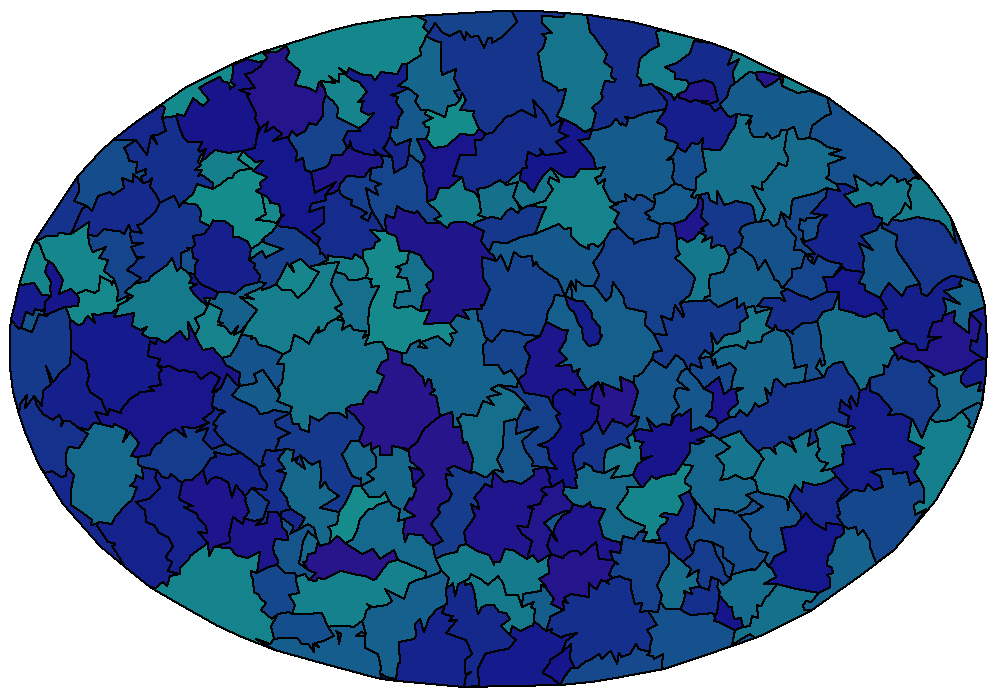
Figure 5. The subdivisions encircled by their borders.

png

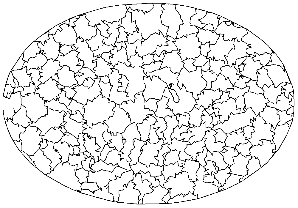
Figure 6. The borders.