Mazes 1.: Background and algorithms

Introduction

This post provides a definition of mazes and proposes a high level approach to create them. This approach will then be utilised to create two maze images.

png

Notes

The raw notebook can be found here. The source of the various maze generating utilities are deposited in this repo.

Goal definition

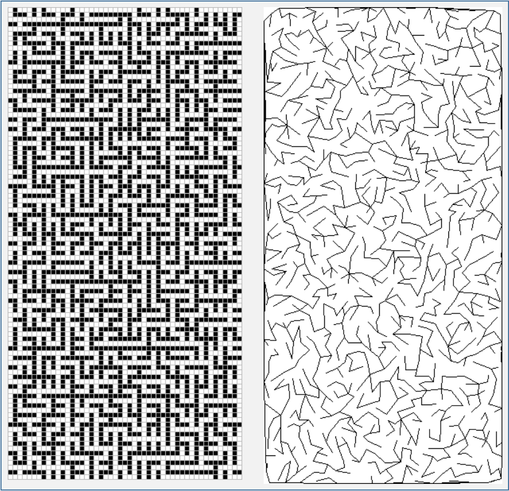
Let us first define what the desideratum is. We would like to have maze images akin to those in Figure 1. There is a rather short sequence of actions to achieve it: print this page off. Then we have one. The issues arise if we wish to posses images that are slightly different in colour, shape, style. Neither of which is changable via the said method.

The goal thus needs rewording. We wish to have maze images of specification of our choice. Alas, there is no method to obtain the desired images as trivial as the the previous one. The only way out seemingly is to create our own utility that produces maze images. Let us restate the goal once more. More importantly, even before starting, we should justify why we choose a certain set of actions, and the effort completing it. It is of paramount importance to recognise that discourse is now about actions not objects.

Task statement

Deliverable: program that creates maze images to given specification
How to achieve it? Write one.
Justification
- we would like to have a variety of maze images (sufficient, isn’t it?)
- the components of the program can be reused in other utilities
- there are no available resources (or they are not flexible enough, incompatible with our tech stack)

Maze definition

The right level of abstraction helps writing reusable code or, even better, utilise units of code that have already been created. right is just as enlightening word as have was. In other terms, it is not especially helpful. By the term right level of abstraction it is meant that the code is applicable to more than just a specific problem, data structure etc. The implementation, on the other hand, is not left blank.

One way to abstract a problem is to identify the common elements across its various instances. The first observation that both panels of Figure 1. contains regions from which it is possible to move to one or more neighbouring one. These regions are either squares (left panel) or pixels or polygons (right panel). There are too neighbouring regions to which it is impossible step (black squares (left panel) and back lines(right panel)).

Three statemets are made based on these observations that define what a maze is.

Let $\mathcal{S}$ a nonempty set of objects. (pixels, regions, etc) $\mathcal{S} \neq \emptyset$
The neighbours of an element of $\mathcal{S}$ is denoted by $\mathcal{N}(s)$ $! s \in \mathcal{N} \\ \mathcal{N}(s) \subseteq \mathcal{S}\setminus \{s\}$

What exactly makes an element a neighbour of an other is irrelevant at this stage. We just formalised the fact that some points are sorrounded by other points irrespective wheter it is possible to move to them.

The linked set of an element, $s$ is denoted by $\mathcal{L}(s)$

\[! s \in \mathcal{S} \\ \mathcal{L}(s) \subseteq \mathcal{N}(s)\]

Again, it is not of our conerns which neighbours are linked. We only stated how these elements may exist.

These three statements above define what a maze is. It is a collection elements and movement may be allowed between neighbouring elements. This definition is also remarkably useless as far as implementation goes. Idealy, a definition would hint at data structures or classes of algorithms that could guide the developer to create the actual piece of software component.

With little effort, the definitions can be transformed in to a more conducive one.

Collect all the pairs of elements that are neighbours. $\mathcal{N} = \bigcup\limits_{s \in \mathcal{S}} \{(s, t): t \in \mathcal{N}(s) \} \subseteq \mathcal{S} \times \mathcal{S}$

If $\mathcal{S}$ is considered to be vertices then $\mathcal{N}$ is the set of edges. $(\mathcal{S}, \mathcal{N})$ is thus a graph on which the possible reachable pairs can be drawn. This graph will be termed as pre-maze.

Collect all edges that are links $\mathcal{L} = \bigcup\limits_{s \in \mathcal{S}} \{(s, t): t \in \mathcal{L}(s) \} \subseteq \mathcal{N} \subseteq \mathcal{S} \times \mathcal{S}$ The set $\mathcal(L)$ will be called links.

A maze, $M$ is the triplet of vertices, all edges and links: $M = (\mathcal{S}, \mathcal{N}, \mathcal{L}) \, .$

Remarks

The $\mathcal{W} = \mathcal{N} \setminus \mathcal{L}$ is called the walls.
If we only concern ourselfs with traversing the maze the tuple $(\mathcal{S}, \mathcal{L})$ contains sufficient information. The neighbours are retained for specific purposes, such as drawing.

In summary, we established that a maze can be represented by graphs. This enables us to use graph algorithms to create mazes. Yet it is abstract enough that we need not care about what the elements are.

Making mazes

The creation of a maze image consists of the following actions

get the specifications (and discuss it!)
define the set of maze objects that would fulfill the specs to the greatest extent
define the pre-maze keeping the specs in mind
apply an algorithm that creates the links
prepare the objects to be drawn
render the maze

My very limited experice confirms that (4.) takes the least amount of resources. Points (2.) and (3.) is where the bulk of the effort is spent. (6.) can sometimes be tedious and it is best to tackle it with experts.

Specifications

Two properties of the mazes will be required

there must exist a path between all pairs of vertices
there must not be cycles of vertices

These are more aesthetic requirements than anything else. The first one is to make sure that a line drawn on the maze will traverses its entire area. The second one is to ensure that always the shortest possible line is drawn between two vertices.

Link generation

Let us assume that we finally have a pre-maze at hand. The specifications dictates us to invoke a graph algorithm that traverses the entire graph reaching each vertex only once. The options are plentiful:

breadth-first search: tends to create river system-like paths
depth-first search: tends to result in pine-like paths
your favourite (minimum) spanning tree algorithm, preferably Kruskal’s algorithm to avoid elongated paths
loop-erased random walk.

Loop erased random walk

We choose the loop erased random walk to create the linkage set. It is expensive due to the moves wasted in loops which are then deleted, but it produces the best looking graphs.

Algorithm

The algorithm in rather simple. Cyle free paths starting from vertices not in the maze are sequentially grown. Once the latest vertex in path is reaches maze the path is attached to it. This is repeated until all the vertices are in the maze. It is constructive to write out the alogrithm in more detail for it guides us implementing it.

\[\begin{eqnarray} &\, &\text{Algorithm } \texttt{MakeLoopErasedRandomWalkLinkage} \\ % &\,& \textbf{Inputs: } (\mathcal{S}, \mathcal{N}) & \quad \text{(pre-maze)} \\ % &\,& \textbf{Output: } \mathcal{L} & \quad \text{(set of maze links)} \\ % &1.& \mathcal{L} \leftarrow \emptyset \\ % &2.& \mathcal{M} \leftarrow \{s\}: s \in \mathcal{S} &\quad \text{(pick a vertex as the first element in the maze)} \\ % &3.& \textbf{while} \, |\mathcal{S} \setminus\mathcal{M}| \neq 0 & \quad \text{(until all vertices are in the maze)} \\ % &4.& \quad \mathcal{P} \leftarrow \emptyset & \quad \text{(path as an indexed set)} \\ % &5.& \quad s \leftarrow \texttt{Choose}(\mathcal{S} \setminus\mathcal{M}) & \quad \text{(choose a vertex which is not in the maze)} \\ % &6.& \quad \textbf{while true} & \\ % &7.& \quad \quad t \leftarrow \texttt{Choose}(\mathcal{N}(s)) & \quad \text{(pick any neighbour)} \\ % &8.& \quad \quad \textbf{if } t \in \mathcal{M} & \quad \text{(neighbour is in the maze)} \\ % &9.& \quad \quad \quad \mathcal{P} \leftarrow \mathcal{P} \cup \{t\} & \quad \text{(add maze vertex to the path)} \\ % &10.& \quad \quad \quad \mathcal{L} \leftarrow \mathcal{L} \cup \{(p_{i}, p_{i+1}), i \in [1, |\mathcal{P}| - 1 ] \} & \quad \text{(create and collate links)} \\ % &11.& \quad \quad \quad \mathcal{M} \leftarrow \mathcal{M} \cup \mathcal{P} & \quad \text{add vertices in the path to the maze} \\ % &12.& \quad \quad \quad \textbf{break} & \\ % &13.& \quad \quad \textbf{end if} & \\ % &14.& \quad \quad \textbf{if } t \in \mathcal{P} & \quad \text{(the path has a loop)} \\ % &15.& \quad \quad \quad i \leftarrow \texttt{FindIndex}(\mathcal{P}, t) & \quad \text{(find the start of the loop)} \\ % &16.& \quad \quad \quad \mathcal{P} \leftarrow \mathcal{P} \setminus \{p_{j}, j > i \} & \quad \text{(remove the vertices in the loop from the path)} \\ % &17.& \quad \quad \quad \textbf{continue} & \\ % &18.& \quad \quad \textbf{end if}& \\ % &19.& \quad \quad \mathcal{P} \leftarrow \mathcal{P} \cup {t} & \quad \text{(append the neighbour to the path)} \\ % &20.& \quad \quad s \leftarrow t & \quad \text{(move forward)} \\ % &21.& \quad \textbf{end while}& \\ % &22.& \textbf{end while} & \\ % &23.& \textbf{return } \mathcal{L}& \\ \end{eqnarray}\]

Notes,

function $\texttt{Choose}$ returns a randomly chosen element of a collection
function $\texttt{FindIndex}$ finds the index of an element in an indexed set

Implementation

The loop erased random walk algorithm is realised in the make_loop_erased_random_walk_maze_links function.

function make_loop_erased_random_walk_maze_links(graph::Graph{T}) where T
    
    # bookkeeping
    statuses = Dict(vertex => 0 for vertex in get_vertices(graph))
    n = length(statuses)
    
    # storage for edges
    edges = zeros(T, (2, n - 1))
    i_edge = 0
    
    path = zeros(T, n)
    
    # initialise maze
    vertex, _ = pop!(statuses)
    
    # main traversing loop
    while length(statuses) != 0
        
        # get a vertex which is not in the maze
        vertex, _ = pop!(statuses)
        path[1] = vertex
        statuses[vertex] = -1
        n_in_path = 1

        # walk
        while true
            # select a neighbour
            neighbours = get_neighbours(graph, vertex)     
            vertex_next = rand(neighbours)
           
            # option i) loop detected
            if (i_loop_start = get(statuses, vertex_next, 0)) < 0

                # convert flag to index in the path
                i_loop_start = - i_loop_start
                
                # reset statuses from the 2nd element of the loop
                for i in i_loop_start + 1:n_in_path
                    statuses[path[i]] = 0
                    path[i] = 0
                end

                # truncate path until the 1st element of the loop
                n_in_path = i_loop_start

                # set 1st loop element as the current vertex and
                # continue the path from there
                vertex = path[n_in_path]
                continue
            end
            
            # option ii) neighbour is already in the maze -> add path to maze
            if get(statuses, vertex_next, 1) == 1
                for i in 1:n_in_path - 1
                    
                    # add edges to the maze
                    source, target = path[i], path[i + 1]
                    edges[1, i_edge += 1] = source
                    edges[2, i_edge] = target

                    # bookkeeping
                    delete!(statuses, source)
                end
                # add last edge
                source = path[n_in_path]
                edges[1, i_edge += 1] = source
                edges[2, i_edge] = vertex_next

                # delete last vertex in path
                delete!(statuses, source)
                # finish path and go to get a new starting verex
                break
            end
            
            # option iii) vertex not in path or maze
            vertex = vertex_next
            path[n_in_path += 1] = vertex
            statuses[vertex] = - n_in_path

        end
    end
    # order the vertices of the links
    edges = sort!(edges, dims=1)

    return edges
    
end

A handful of remarks on the implementation are in order.

A graph is the input.
The output is the links, the set of edges which define the possible moves in the maze.
The graph must be connected. It is not possible to link up all of the vertices otherwise.
The vertices of the graph must be hashable. Other than that, they can be anything.
The get_vertices function creates an array of the vertices of the graph.
The get_neighbours function returns the neighbours of a vertex in the input graph.
The exact implementation of these functions depends on the type of the input graph. The random walk algorithm itself is concerned not how these goals are achieved. It only requires a certain behaviour of the functions. By doing so, the algorithm is not tied to a specific data structure. On the other hand, having these to two functions implemented is the bare minimum what can be expected from any graph code suite.
The crux of implementation is the statuses hash map.
- The keys are the vertices which are not linked to the maze yet.
- If the vertex is in a path being grown its value is minus its position in the path. This is to find loop erasure points in $O(1)$ time.
- If a vertex is not in the path being grown its value is zero.
- If a vertex is in the maze the default value of unit is returned from the map.

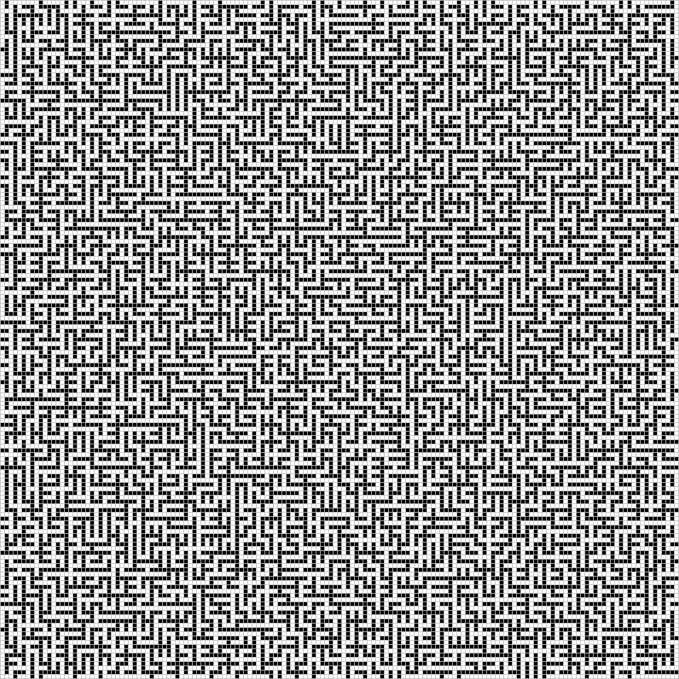
Example 1.: Square maze

1. Specifications

We set out to create a maze akin to the left panel of Figure 1. The vertices of the maze are the points of a reactangular grid.

2. Objects

The elementary geometric object of the square maze is a square which are arranged in a grid. This grid implemented as the RectangleGraph structure. It only containts the number of rows, columns and vertices of the grid across which the maze spans. It is a subtype of the Graph structure whose role is to ensure type consistency.

abstract type Graph{T} end
 
 struct RectangleGraph{Int} <:Graph{Int}
     n_rows::Int
     n_colums::Int
     n_vertex::Int
 end
 RectangleGraph(n_rows::Int, n_columns::Int) = RectangleGraph(n_rows, n_columns, n_rows * n_columns)

3. Pre-maze

The pre-maze is only defined implicitly. The get_neighbours function determines the indices of gridpoints (vertices) in the 4-connectivity neighbourhood of a given vertex. Alternatively, these the neighbours could be precomputed and stored. Since they can be calculated cheaply, they are generated on demand as opposed using up space for storage.

pre_maze_rectangle = RectangleGraph(80, 80)
# RectangleGraph{Int64}(80, 80, 6400)

4. Generation of the links

The random walk algorithm is called on the pre-maze yielding the set of links. Each link is a coordinate pair of grid points.

links_rectangle = make_loop_erased_random_walk_maze_links(pre_maze_rectangle)

#     2×6399 Matrix{Int64}:
#     4700  4621  4621  4622  4623  4544  …   70  5992  2798  2784  459  5336
#     4701  4701  4622  4623  4624  4624     150  6072  2799  2864  539  5416

5. Transformation to geometrical objects

The abstract maze is transformed to a set of geometrical object. Each vertex and edge is represented by a square. This means the following transformations

vertices:
- $i \rightarrow (i_{col}, i_{row})$ (convert vertex indices to grid coordinates)
- $(i_{col}, i_{row}) \rightarrow (2 i_{col}, 2 i_{row})$ (make space for the edges)
edges:
- $(i, j) \rightarrow ((i_{col}, i_{row}), (j_{col}, j_{row}))$ (convert vertex indices to grid coordinates)
- $((i_{col}, i_{row}), (j_{col}, j_{row})) \rightarrow (i_{row} + j_{row}, i_{col} + j_{col})$ (calculate edge square coordinates)

This is done by the convert_links_to_points_rectangle function. It outputs the grid coordinates of those squares which correspond to vertices or links. Strictly speaking, the shapes to be drawn need not to be squares.

x, y = convert_links_to_points_rectangle(
    links_rectangle,
    pre_maze_rectangle.n_row,
    pre_maze_rectangle.n_column
)
nothing

6. Rendering

The create_maze_bitmap_rectangle makes a 2D bitmap of greyscale colours using the previously computed coordinates. The vertices and the links are rendered as white squares. The walls will show up as black squares. Each of them is the most tastefully separated from its neighbours by gray borders.

img = create_maze_bitmap_rectangle(
    x, y,
    pre_maze_rectangle.n_row,
    pre_maze_rectangle.n_column, 5, 1
)
# then save img

png

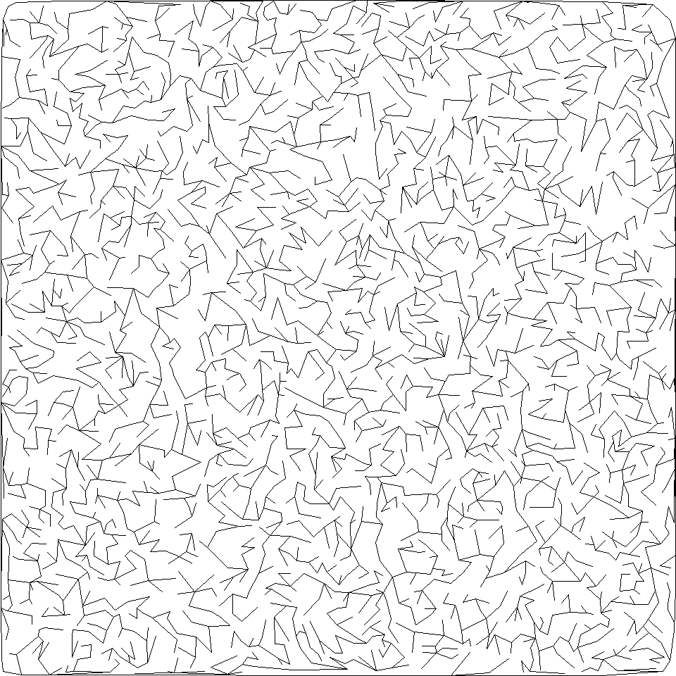
Example 2: Deluanay maze

1. Specification

We wish to create a graph where the paths are in the forms connected polygons.

2. Object

The objects are adjacent triangles which have two vertices in common. The removal of some of the shared side leads to the desired polygon effect. The TriGraph structure encapsulates all pieces of information that span the pre-maze.

graph is be the graph of the adjacent triangles
mapping is a bijection between the index pairs of the adjoining triangles and the indices of points of the side along which they are connected
tri is a triangulation object from which the previous are derived. It is retained in the structure for it is needed for the drawing.

struct TriGraph{T} <: Graph{T}
    "`graph::Dict{T, Array{T, 1}}` triangle connectivity"
    graph::Dict{T, Array{T, 1}}
    "`mapping::Dict{Tuple{Int, Int}, Tuple{T, T}}` triangle-pair--side mapping"
    mapping::Dict{Tuple{Int, Int}, Tuple{T, T}}
    "`tri::DelaunayTriangulation.Triangulation`: triangulation"
    tri::DelaunayTriangulation.Triangulation
end

3. Pre-maze

The bulk of the effort, again, is consumed by creating the pre-maze. Naively, a Delaunay triangulation of any randomly sampled points in two dimensions would be sufficient. This, however, may lead to triangles that are too small to be rendered correctly at the available resolution. I.e. some paths may appear as closed if the line width is comparable to distance between the points whose connecting edge is removed.

3.1 Sampling of points

It thus required that all distances are greater than a certain limit, $\rho$ in order to avoid generating small triangles. This implies that a cirle of radius $\rho / 2$ centred on each point cannot contain other points. In other words, the points are replaced by circles. We are thus tasked with placing circles in an area which is the sphere packing problem.

There is a plethora of exact and approximate solutions to this problem. The former ones fall in two broad categories

physical methods: the speres are considered to be particles which are propagated according to certain laws of motion
mathematical: mathematical constructs are utilised to obtain the set of suitably positioned spheres

Randomised sampling belongs to the second group. This, yet again, separates in two groups

bottom-up: the points are incrementally added. Each time a point that is far enough from all of the previous points. Rejection sampling is the phrase that springs up in one’s mind and it is immediately discarded in this post. Due to the restricted amount time that is available to the author os these lines, an approach is chosen which relies on static data structures.
top-down: a set of random points is created from which points are discarded until all distances are greater than the required limit.

3.1.1. Initial sampling

The 2D range search can have an $O(N^{2})$ complexity if the search radius is comparable to the extent of the point set. Regions of high point density can also lead to degradation of the performance. Choosing the correct search radius is thus crucial.

The point coordinates will, some point, be scaled to the canvas coordinates taking the resolution into account. The relationship between the drawing line width and the size of the pysically available canvas will eventually determine the number of points.

Let

$h, w$ the height and the width of the draw area
$l = \sqrt{h \cdot w}$ the charateristic size of the draw area.
$d$ the line width in the same units as $l$
$\rho = m d$ is the minimmum required separation; a small multiple of the line width
if $h$ and $w$ are roughly equal and much larger than $\rho$ then
$N \approx \left[ \frac{l}{m d} \right]^{2}$ points can be placed on the canvas

The questions is how many points can be placed on a canvas of given size and a given line width so that a specified portion of the points will be closer to each other than the required limit. The nearest neighbour distances are spread according to the Rayleigh distribution

\[P(r \leq R) = 1 - \exp\left[ - \frac{R^{2}}{2 \sigma^{2}} \right] \\ \sigma^{2} = \frac{A}{2 \pi N} = \frac{l^{2}}{2 \pi N}\]

where $r$ is the nearest neighbour distance $A$ is the area of the point set, $N$ is the number of points.

\[p = P(r \leq m d ) = 1 - \exp \left[ - \frac{m^{2} d^{2}}{2} \frac{2 \pi N}{l^{2}} \right]\]

From which

\[N = - \left[ \frac{l}{md} \right]^{2} \frac{\ln(1 - p)}{\pi }\]

The function calc_2D_points_sample_size estimates the maximum allowed number of points.

Nearest Neighbour Graph

A kD-tree is constructed from the points ($O(N\log(N))$). The pairs which are closer than the minimum required distance are found by a range search. The average cost is $O(\log(N))$ whilst the worst case cost is $O(N^{2})$. By limiting the maximum number of points we have already reduced the possibility of this happening so.

The KDTree structure of the NearestNeighbours package is used to construct the graph which is implemented in the create_neighbour_graph function.

Thinning

The aim, still, is to create a set of dense points with a required minimum distance between them. A simple algorithm is outlined below to obtain a set specified so. Let $\mathcal{S} \subset \mathbb{R}^{2}$ be a non-empty set of points in the plane.

Let $d$ be the $L_{2}$ distance over $\mathbb{R}^{2}$. Then collect all pairs of points whose distance is smaller than the limit: $E \subseteq \mathcal{S}^{2} = \left\{ s, t \in \mathcal{S}: d(s, t) < \rho \right\} \, .$

$(\mathcal{S}, E)$ is then a graph (it is most likely to be a forest). If the graph has no edges then all points are separated by the desired amount. The task of creating a point set is in essence is reduced to solving a trivial graph problem. The question is in what order the edges should be removed. We will eliminate them is descending along their degrees in order to retain the most points.

Algorithm

$\texttt{ThinGraph}$ is the algorithm that marks the points removal of which results in a set in which all pair distance are not less than the minimum required limit.

\[\begin{eqnarray} &\, &\text{Algorithm } \texttt{ThinGraph} \\ % &\,& \textbf{Inputs: } (\mathcal{S}, E) & \quad \text{(neighbourhood graph)} \\ % &\,& \textbf{Output: } \mathcal{R} & \quad \text{(set of vertices to remove)} \\ % &1.& \mathcal{R} \leftarrow \emptyset \\ % &2.& \mathcal{V} \leftarrow \texttt{SelectVertices}(\mathcal{G}, m) & \quad \text{(select vertices of large degrees)} \\ % &3.& \mathcal{V} \leftarrow \texttt{OrderVertices}(\mathcal{V}) & \quad \text{(make ordered set)} \\ % &4.& \mathbf{while} |\mathcal{V}| \neq 0 & \quad \\ % &5.& \quad s \leftarrow \texttt{PopFirst}(\mathcal{V}) & \quad \text{(remove vertex of largest degree)} \\ % &6.& \quad \mathcal{R} \leftarrow \mathcal{R} \cup \{ s \} & \quad \text{(save vertex)} \\ % &7.& \quad \mathbf{for} \, t \in \mathcal{N}(s) & \quad \text{(investigate neighbours in the vertex)} \\ % &8.& \quad \quad \mathbf{if} \, t \notin \mathcal{V} & \quad \text{(vertex has already been removed)} \\ % &9.& \quad \quad \quad \mathbf{continue} & \\ % &10.& \quad \quad \mathbf{end} & \\ % &11.& \quad \quad E \leftarrow E \setminus \{ (s, t) \} & \quad \text{(remove edge from the graph)} \\ % &12.& \quad \quad \mathbf{if} \, \mathrm{deg}(t) < m & \quad \text{(has allowed number of edges)} \\ % &13.& \quad \quad \quad \mathcal{S} \leftarrow \mathcal{S} \setminus \{ t \} & \quad \text{(vertex is no longer of interest)} \\ % &14.& \quad\quad \mathbf{end} & \\ % &15.& \quad \mathbf{end} & \\ % &16.& \mathbf{end} & \\ &23.& \textbf{return } \mathcal{R}& \\ \end{eqnarray}\]

A handful of remarks on the algorithm

$\texttt{SelectVertices}$ selects those vertices whose degree is greater than a limit. This limit is one in this problem.
$\texttt{OrderVertices}$ orders the vertices in a descening sequence according to their degrees
We immediately see that a data structure is needed which
- is ordered
- provides $O(1)$ lookup
- is mutable

Implementation

The thin_graph function implements the edge removal algorithm.

function thin_graph(graph::DictGraph{T}, max_degree::Int) where T

    # vertex degree mapping
    degrees = Dict(
        vertex => length(get_neighbours(graph, vertex))
        for vertex in get_vertices(graph)
    )
    # select vertices which are in more than the allowed edges
    degrees = Dict(
        vertex => degree for (vertex, degree) in degrees if degree > max_degree
    )
    vertices = collect(keys(degrees))
    degrees = [degrees[vertex] for vertex in vertices]

    # sort the selected vertices in descending order acc. to their degrees
    idcs = sortperm(degrees, rev=true)
    degrees = OrderedDict(zip(vertices[idcs], degrees[idcs]))

    # remove vertices -- one pass is enough
    to_remove = Set{T}()
    for (s, _) in degrees
        
        # explicit vertex deletion
        # for some reason, we need to reference `degrees`
        # otherwise the vertex is not deleted
        if haskey(degrees, s)
            delete!(degrees, s)
            push!(to_remove, s)
        end

        # implicit vertex deletion through edges
        for t in get_neighbours(graph, s)
            if haskey(degrees, t)
                deg_curr = degrees[t] -= 1
                if deg_curr <= max_degree
                    delete!(degrees, t)
                end
            end
        end
    end

    collect(to_remove)
end

Notes,

the central data structure is the degrees OrderedDict which fulfills all three requirements
it stores the degrees of the vertices of the neighbour graph

height_canvas = 960
width_canvas = 960
xy = sample_drawing_points_2d(4000, height_canvas, width_canvas, 2, 4)

#    2×2869 Matrix{Int64}:
#     459  349  377  943  880  735  304  330  …  489  584  525  906  524  133  842
#     122  199   55  768  877  334  870  930     286  271  806  581  775    6  926

tri_graph = TriGraph{Int}(xy)

#    TriGraph{Int64

4. Links

The links are generated with the make_loop_erased_random_walk_maze_links function. A links is the pair of the the indices of two adjoining triangles whose shared side is removed to create a path. Again, it only requires that the get_neighbours function is defined for this particular type of graph.

links = make_loop_erased_random_walk_maze_links(tri_graph)

#    2×5636 Matrix{Int64}:
#     3275  3275  2021  2021  2022  2153  …  4555  458  2999   241  4724  4496
#     4700  5383  5383  2022  2153  5452     4759  459  3847  1711  4970  5068

5. Transforming to geometrical objects

The select_sides_to_draw_tri gathers those triangle sides which are retained. E.g. the connectivity of two triangles is represented by removing their shared sides. The geometric object to draw are therefore not triangles but straingth lines.

sides_to_draw = select_sides_to_draw_tri(tri_graph, links)

#    2831-element Vector{Vector{Int64}}:
#     [433, 211, 425, 230]
#     ...

6. Rendering

A bitmap of lines is constructed through rasterisation using the excellent SimpleDraw library.

img = draw_lines_on_bitmap(height_canvas, width_canvas, sides_to_draw, 1)

#    960×960 Matrix{Int64}
#    then save

png

Conclusion

We have defined mazes as graphs and implemented a generator of them agnostic of what objects constitute the actual maze. The creation of mazes requires the effort to be concentrated at making a mathematical representation of the objects and their preparation for rendering.