Mazes 2.: Picture mazes

Introduction

This post builds on the first part of maze posts where a formalism and a procedure were introduced to create maze images. We are going to turn pictures to mazes. The algorithms purposed so are discussed at length.

Notes

The raw notebook can be found here. The source of the various maze generating utilities are deposited in this repo.

Recycling

The previous blog proposed that the creation of a maze is comprosed of six stages.

specification
defining the objects
from which the pre-maze is assembled
the links of the maze are marked
preparing the objects to be drawn according to the links
the maze is rendered

At least two stages require no development

1. the already implemented loop-erased random walk algorithm will select the links
1. the primitive drawing subroutine will render the maze

1. Delaunay maze

1.1. Specification

We wish to turn the image in the lest panel of Figure 1. to a Delaunay maze.

1.2. Maze objects

The maze objects are triangles which are spanned by the non-blank pixels of the original image.

1.2.1. Image preparation

The maximum width and the height of the image given in pixels are constrained by the size and the resolution of the final maze. I.e. the final maze image has practical limits on its size. The finite resolution of the raster image defines the physical width of a drawn line. The ratio of one fifth between line width and minimum spacing between parallel lines is aesthetically pleasing according to the scribbler of these lines. Therefore, if

$l = \sqrt{w h}$ is the approximate width of the maze
$d$ is the line width
$m=5$ is separation between lines in multiples of the line width then a maximum $N \approx l / (m + 1) d$ of image points are allowed in one dimension of the maze image.

The starting image then either needs to be not larger than $N \cdot N$ or it requires downsampling using your favourite method.

Downsampling also condenses the information encoded in the image which are hopefully recreated by the maze lines. There will be more points, thus triangles, thus lines in the darker regions of the original image. Where the photograph is lit, the lines will be sparse. The role of shading is transferred from hints of grey to density of lines. Figure one shows these there images. Please note that the original image is resized too.

The original greyscale photograph needs to be binarised in order to create the points over which the triangles are spanned. The Again, books have been written on binarising images. Choice is yours, don’t be grey.

# load image
img = load("<path-to-image>")

img = imresize(img, ratio=0.25)

# quantise colours
img_binary = binarize(img, AdaptiveThreshold())
points_all = convert(Array{Int}, Gray.(img_binary))

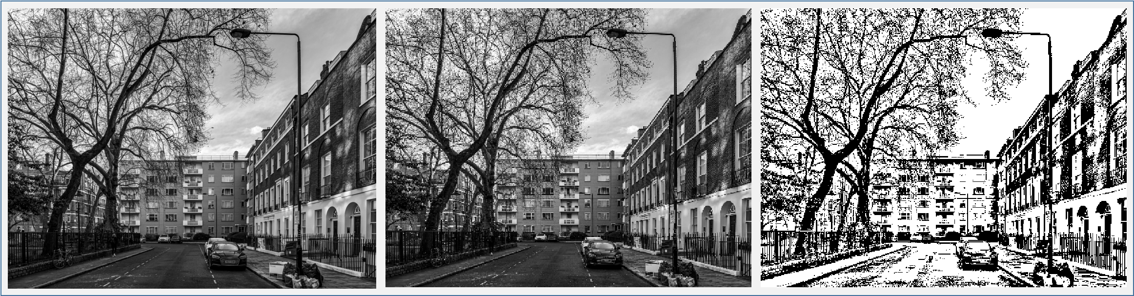png Figure 1. The original (left panel), the resized (middle panel) and the binary images (right panel).

1.3. Pre-maze

All of the Delaunay maze code written in Part 1. can be reused once there is a pointset across which the triangulation spans.

The extract_coords function is instructed to return the 2D grid indices of the black points in an image. The binary image is in the points_all variable.

xy = extract_coords(points_all, 0)

#    2×69578 Matrix{Int64}:
#     5  6  7  11  14  16  17  25  26  33  …  353  354  355  356  357  358  359
#     1  1  1   1   1   1   1   1   1   1     480  480  480  480  480  480  480

The coordinates are then scaled with a constant to create space for the line to be drawn on a bitmap.

width_line = 1
factor = 5

xy .*= (width_line + factor)


#    2×69578 Matrix{Int64}:
#     30  36  42  66  84  96  102  150  156  …  2124  2130  2136  2142  2148  2154
#      6   6   6   6   6   6    6    6    6     2880  2880  2880  2880  2880  2880

4–6. Links, drawing object preparation, rendering

Creating and drawing the maze is a trivial affair with the functions developed in the previous post.

# create a Deluanay graph
tri_graph = TriGraph{Int}(xy)

# make a maze
links = make_loop_erased_random_walk_maze_links(tri_graph)

# mark up triangle side to draw
ptd = select_sides_to_draw_tri(tri_graph, links)

# render image
img_maze = draw_lines_on_bitmap(5000, 6000, ptd, 1)

The entire Deluanay maze is shown in Figure 2. along with a detail. The lightness of the original photograph has indeed been translated to triangle densities. The full size maze can be found here.

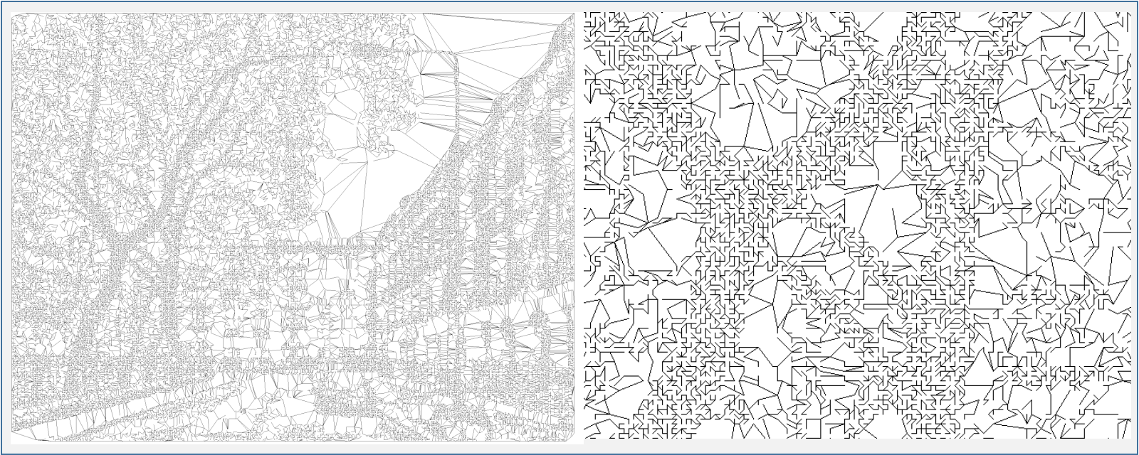png Figure 2. The Delaunay maze (left panel) and a detail (right panel).

2. Rectangle maze

2.1. Specification

Each black pixel is replaced by a rectangle. The vertices of the maze are these rectangles and the blank areas enclosed by them. The links are created by removing the walls of the rectangles.

2.2. Maze objects

2.2.1. Object types

There are two kinds of objects. The grid rectangles with which the black pixels are subtituted as shown in the left and middle panels of Figure 4. The location of these are simply given by their 1D or 2D grid indices. They will be identified by the former one in the pre-maze.

These rectangles – and the image borders – enclose single or connected blank pixels of the image. They form the of other type of objects which will be called components. The collection of the grid rectangles can be viewed as the foreground and the regions of connected white ones as the background. In the image segmentation parlance, the latter ones are called connected components. These are of irregular shape and can neighbour a wast range of number of black pixels, yet they correspond to a single vertex in adjacency graph of the maze.

2.2.2. Labeling of connected components

We thus need to identify which blank pixel belongs which connected component. We could use purely graph based algorithms, such as exhaustive enumeration e.g. depth or breadth first search. Alternatively, numerical image segmentation procedures, such as the watershed algorithm may be invoked. Halfway between them lies the Hohsen–Kopelman connected component labeling algorithm. It is implemented in the label_connected_components_image function.

It takes a binary image as an input where the “black” pixels are marked. It then performs the two pass algorithm assigning negative component labels to the blank areas. It is done to avoid clashing with the grid indices of the black pixels.

Note, there are julia packages of various maturity which offer an implementation of the algorithm utilised here. I have chosen to write my own, label_connected_components_image! which is not necessarily a good practice, even if it only took a little time and I derived much joy from it. Which happens to by exactly my utility function. The result of this function is a 2D array where the foreground pixels are set to zero and the positions corresponding to connected coponents have negative values. The right panel of Figure 3. provides a view of the connected components coloured in shades of blue.

# load image
img = load("<path-to-image>")

img = imresize(img, ratio=0.25)

# quantise colours
img_binary = binarize(img, AdaptiveThreshold())
points_all = convert(Array{Int}, Gray.(img_binary))

img_labels = points_all .+ 0
Maze.label_connected_components_image!(img_labels, 0)

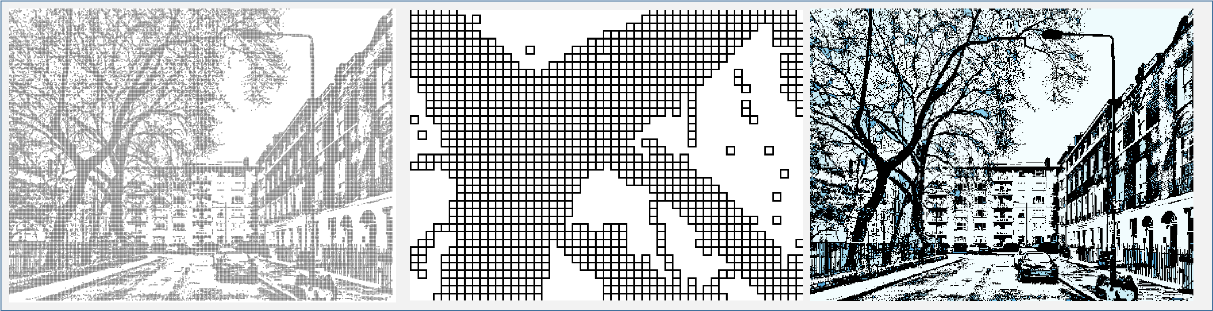png Figure 3. The black pixels replaced by squares (left panel), detail (middle panel), the connected components (right panel).

3. Pre-maze

3.1. Algorithm

Once all of the vertices, let they be standalone grid rectangles or components are labeled, their connectivity is determined. This is done in a single pass where only the grid rectangles are examined. We know that they are either connected to each other or to the components. Two components cannot share a border because they would form a single larger component.

3.2. Implementation

The ImageGridComponentGraph is a convenience structure to collate the information on the objects of the image. Itc constructor takes a labeled image (img_labels) as an argument. The connectivity is stored in a DictGraph structure (graph) introduced in the previous post.

struct ImageGridComponentGraph{Int} <: Graph{Int}
    "`graph::Dict{Int, Array{Int, 1}}`: component connectivity"
    graph::Dict{Int, Array{Int, 1}}
    "`image_components::Array{Int, 2}`: 2D array of labeled image components"
    image_components::Array{Int, 2}
end

The constructor simply iterates over all pixels. It only examines the background pixels of the labeled image. The foreground regions are defined implicitly by the background.

take a backround pixel
retrieve its neighbours
loop over the neighbours
1. if the neighbour is background use its grid index as a vertex
2. otherwise use the component label
save edge to the graph

function ImageGridComponentGraph(x::Array{Int, 2})

    n_row, n_col = size(x)
    
    # for lookup
    grid = RectangleGraph(n_row, n_col, n_row * n_col)

    connectivity = DictGraph{Int}()
    
    # examine each pixel
    for j in 1:n_col
        for i in 1:n_row
       
            # skip foreground (labeled components)
            if x[i, j] != 0
                continue
            end

            # calculate 1D index which will be the vertex
            source = index_2d_to_1d_grid(i, j, n_row)

            # get neighbours
            targets = get_neighbours(grid, source)

            # add to graph
            for target in targets
                # if the neighbour is a background pixel use its grid index
                # otherwise use the component label
                target = (x[target] == 0) ? target : x[target]
                push!(connectivity, source, target)
                push!(connectivity, target, source)
            end

        end
    end
    ImageGridComponentGraph(connectivity, x)

end

4. Links

The loop erased random walk algorithm is yet again invoked to select a set of edges of the image grid graph. Again, one only needs to implement the get_neighbours function for the ImageGridComponentGraph structure which is barely more than a line.

function get_neighbours(graph::ImageGridComponentGraph, vertex::Int)
    get_neighbours(graph.connectivity, vertex)
end

links = make_loop_erased_random_walk_maze_links(graph)

5. Drawing object preparation

There are two kinds of links. Those that connect grid rectangles and those that communicate between grid rectangles and components. The grid rectangles are connected through a single shared side. This side is not rendered so that a visual path is created in the maze image.

A component connected to a grid rectangle can be adjacent to it at least one and at most four sides. The latter happens when the rectangle is an enclave in the component. The possibility of having more than a single side to remove needs to be dealt with.

select_sides_to_omit_component considers these two cases. The first is trivial to handle.

the two 1D grid indices are fed to the get_shared_sides_rectangle function which
1. forms the difference of the indices
2. from which the position of the shared side is determined
which is then saved

The second possibility is just a little more complicated. We will use the fact that the component vertices are the component labels.

the 1D grid indices of the neighbours of the grid rectangle are retreived
they are randomly permuted
loop over the 1D indices
1. check whether the component image value at the current index is equal to the target index
2. if so,
  1. save index
  2. stop iteration

The random permutation is to ensure that all shared sides are deleted with equal probaility.

function select_sides_to_omit_component(
        x::Array{Int, 2},
        links::Array{Int, 2}
    )
    n_row, n_col = size(x)
    grid = RectangleGraph(n_row, n_col)

    sides_to_omit = DictGraph{Int}()

    # loop over all links to find connecting sides
    # `source` is always a grid rectangle
    for (target, source) in eachcol(links)

        # if both are grid rectangles
        if source >= 1 && target >= 1
            
            # get at which (N/E/S/W) sides the two grid rectangles meet
            side_source, side_target = get_shared_sides_rectangle(
                source, target, n_row
            )

            # save which side will not be rendered
            push!(sides_to_omit, source, side_source)
            push!(sides_to_omit, target, side_target)

        # `source` is a grid rectangle, `target` is a component
        elseif source >= 1 && target < 0

            # the neighbours are given in grid 1D indices
            for neighbour in shuffle(get_neighbours(grid, source))
                    
                # choose the first neighbour which matches the index of the component
                if x[neighbour] == target
                    side_source, side_target = get_shared_sides_rectangle(
                        source, neighbour, n_row
                    )
                    # only save the grid rectangle side
                    # (components are rendered indirectly)
                    push!(sides_to_omit, source, side_source)
                    break
                end
            end
        else
            throw(ErrorException("something"))
        end

    end

    return sides_to_omit.graph
end

6. Rendering

All foreground rectangles are looped over and their retained lines are plotted yielding the astoundingly beautiful – and this is an understatement – left panel of Figure 4. The full resolution grid maze is stored here.

lines = select_lines_to_draw_component(graph, links)
img_rect = draw_lines_on_bitmap(2500, 2500, lines, 1)

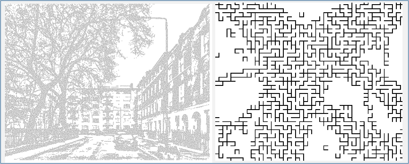png Figure 4. The entire grid maze (left panel), detail (right panel).