Introduction
The similarity of popular songs is quantified based on their perceived loudness in this blog post. The first part of the twin entries transformed mp3 waveforms to smooth time series of loudness. These were brought to a scale whose minimum was the normal auditory limit and its maximum was the pain threshold – averaged over all musical tastes. The loudness progressions were represented by a Legendre polynomial series expansion.
We first define what is meant by likeness of two songs. A suitable mathematical expression is then sought to quantify this notion. With the help of it, we will finally savour various flavours of group similarity.
Note
The raw notebook is located in this folder. The sripts utilised therein are deposited in this repository.
Data
We will concern ourselves with the oeuvre of Adele. The songs released by the artist only on her studio albums are the material of this investigation.
Data preparation
The songs were recast as smoothed perceived loudness time series in the previous post. Most of the transformations are reused here with a few minor differences.
Smoothing
It migth be of interest for those technically inclided that the expansion coefficients were determined by approximating the overlap integral between the Legendre polynomials the subsampled series with the trapezoidal rule over the Chebysev nodes. This way, a more accurate, higher order smoothing is obtained by doing away with the faux oscillations due to Runge’s phenomenon.
Trimming
The first and last three seconds of each song were removed from in order to avoid spurious increase of the overlap due to the bracketing silent or barely audible sections.
Loudness again
The previously introduced loudness scale is an absolute one. Whilst all values on it are directly comparable i.e. 25 is twice as quiet as 50, the relative differences now depend on the values from which they are derived. For example, $10 = 80 - 70$ and $10 = 40 - 30$ does not anymore reflect the same loudness ratio.
Series
A handful of properties of the time series are summarised here to aid drive along the main direction of the present discussion and explore some cul-de-sacs. Let all series be defined over the same domain and codomain:
\[\begin{eqnarray} !A, B & \in & \mathbb{R}: - \infty < A < B < \infty \quad & \text{(finite domain)} \\ % \mathcal{D} & = & [A, B] \quad & \text{(domain)} \\ % ! U, V & \in & \mathbb{R}: 0 \leq U < V < \infty \quad & \text{(non-negative finite function values)} \\ % \mathcal{R} & = & [A, B] \quad & \text{(codomain)} \\ % \mathcal{F} & = & \left\{ f : [A, B] \rightarrow [U, V] \right\} \quad & \text{(functions of interest)} \end{eqnarray}\]The domain is the closed–closed interval betwen -1 and 1 in our case, $[A = -1, B = 1]$. The codomain spans between zero and hundred, $\mathcal{R} = [U = 0, V = 100]$.
Let $f$ and $g$ defined over this domain and codomain. Both of them are expanded with our choice of Legendre basis. \(\begin{eqnarray} \forall x \in \mathcal{d}: f(x) & = & \sum\limits_{k=0}^{K} a_{k}P_{k}(x) \\ \forall x \in \mathcal{d}: g(x) & = & \sum\limits_{k=0}^{L} b_{k}P_{k}(x) \end{eqnarray}\)
The orthogonality of the Legendre polynomials comes handy too:
\[\begin{eqnarray} \int\limits_{x=-1}^{1}P_{k}(x)P_{l}(x) \mathrm{d}x & = & \frac{1}{2k + 1} \delta_{kl} \end{eqnarray}\]The expansion coefficients define a vector in $\mathbb{R}^{K}$ and $\mathbb{R}^{L}$. Both vectors are made to be in the same space by padding the higher dimensions of the lower order one with zeros:
\[\begin{eqnarray} ! K, L & \in & \mathbb{N} : 0 < K \leq L < \infty \quad & \text{(number of the expansion coefficients)} \\ % \mathbf{a}, \mathbf{b} & \in & \mathbb{R}^{L + 1} \quad & \text{(vectors)} \\ % (\mathbf{a})_{i} & = & \begin{cases} a_{i - 1} & \text{ if } i \leq K \\ 0 & \text{ if } f K < i \leq L \end{cases} \quad & \text{(pad dimension absent)} \\ % (\mathbf{b})_{i} & = & b_{i - 1} \quad & \text{(higher order expansion)} \end{eqnarray}\]The subsampled and the Legendre smoothed series are shown in Figure 1. The expansion order was set to one hundred for all songs. This gives a resolution of 3.6 seconds between adjacent peaks at a mean song length of three minutes.
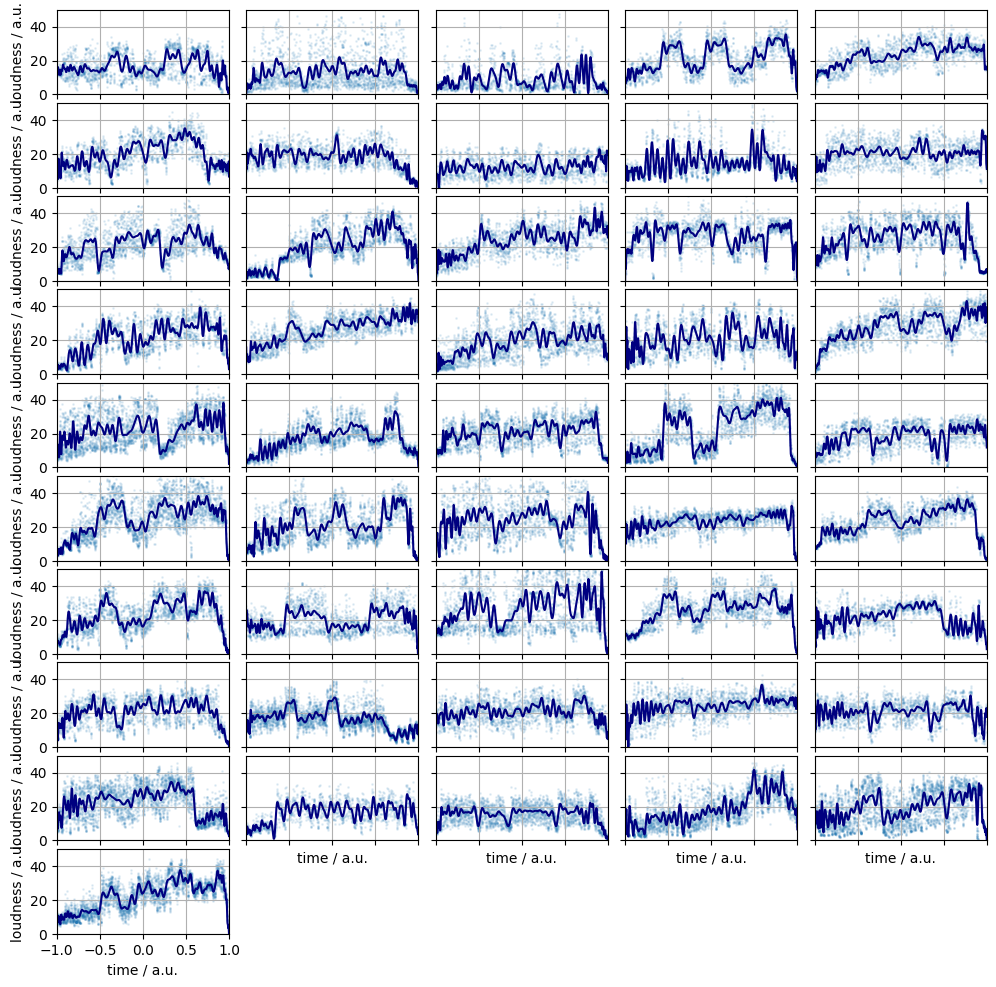
Figure 1. The subsampled loudness time series (pale blue dots) and their Legendre smoothed counterparts (bark blue lines).
Similarity
Two series are similar if they have close loudness values which follow a like pattern. In other words, the progression of the values during a period in one series can be observed in the other one around the same time and position.
Quantifying similarity
Mean squared error
The normalised mean squared error is zero when the two series are identical. Its drawback that is sensitive to shifts: If two loudness progressions are similar, but changes in one lag behind those of the other this measure quickly goes up in value. This will indicate dissimilarity contrary our perception and the definition. See the top panel of Figure 1. as an example.
Cul-de-sac with a view 1.
The mean square error is related to the Euclidean norm of the difference vector of the coefficient vectors. One can prove it by either through the orthogonality of the basis functions, or, equivalently, recalling Parseval’s identity.
\[\begin{eqnarray} D(f, g) & = & \frac{1}{B - A}\int\limits_{x=A}^{B} (f(x) - g(x))^{2} \mathrm{d}x \quad & \text{(integral of the squared error)} \\ % & = & \frac{1}{B - A} \left[ \sum\limits_{k=0}^{N}a_{k}^{2} + \sum\limits_{k=0}^{N}b_{k}^{2} - 2 \sum\limits_{k=0}^{N}a_{k}b_{k} \right] \quad & \\ % & = & \frac{1}{B - A} || \mathbf{a} - \mathbf{b}|| \quad & \end{eqnarray}\]Because of the domain and the codomain of all functions, $[A, B], [U, V]$, are identical, the maximum possible mean sqaured error is $(V - U)^{2}$. Normalising by which the most dissimilar series will have a distance of unit.
Correlation
The various correlation coefficients only consider trends but not the location by design. For instance, Pearson’s:
\[\begin{eqnarray} \varphi(f, g) & = & \frac{ \int\limits_{x=A}^{B}(f(x) - \bar{f})(g(x) - \bar{g}) \mathrm{d}x }{ \left[ \int\limits_{x=A}^{B}(f(x) - \bar{f})^{2} \mathrm{d}x \right]^{\frac{1}{2}} \cdot \left[ \int\limits_{x=A}^{B}(g(x) - \bar{g})^{2} \mathrm{d}x \right]^{\frac{1}{2}} } \quad & \text{(Pearson correlation coefficient)} \\ % \{f, g \} & \ni & h: \bar{h} = \int\limits_{x=A}^{B}f(x)\mathrm{d}x \quad & \text{(means)} \end{eqnarray}\]The middle panel of Figure 2. juxtaposes two series which have Pearson coefficient of unit. They are however not similar, one belonging to a hypothetical song which is quiet throughout whilst the other one is loud.
Cul-de-sac with a view 2.
A certain advantage of the Pearson correlation coefficient that it can be calculated in $\mathcal{O}(1)$ time from the expansion coefficients:
\[\begin{eqnarray} \varphi(f, g) & = & \frac{ \sum\limits_{k=1}^{L}a_{k}b_{k} }{ \left[ \sum\limits_{k=1}^{L}a_{k}^{2} \right]^{\frac{1}{2}} \cdot \left[ \sum\limits_{k=1}^{L}b_{k}^{2} \right]^{\frac{1}{2}} } \, . \end{eqnarray}\]Let us define the demeaned coefficient vectors: \(\begin{eqnarray} ! \mathbf{a_{1}}, \mathbf{b_{1}} & \in & \mathbb{R}^{L} \quad & \\ % (\mathbf{a_{1}})_{i} & = & (\mathbf{a})_{i + 1} \quad & \text{(drop mean)} \\ % (\mathbf{b_{1}})_{i} & = & (\mathbf{b})_{i + 1} \quad & \text{(drop mean)} \\ \end{eqnarray}\)
Then the Pearson correlation is the angle between these two vectors:
\[\begin{eqnarray} \varphi(f, g) & = & \frac{\mathbf{a_{1}} \cdot \mathbf{b_{1}}}{||\mathbf{a_{1}}|| \cdot ||\mathbf{b_{1}}||} = \phi(\mathbf{a_{1}} ,\mathbf{b_{1}}) \end{eqnarray} \, .\]Dynamic time warping distance
The dynamic time warping distance (DTW )is able to link multiple points from one curve to multiple points on the other one. Through this way, features spanning more than a single point can be matched and compared.
The continuous DTW allows, similarly, for pairing of subdomains of different lengths between the two series. This is achieved by stretching or contracting subsections of the two domains ($x$ values) with the functions $\alpha(x)$ and $\beta(x)$.
\[\begin{eqnarray} (1) & : & ! \alpha, \beta: \mathcal{D} \rightarrow \mathcal{D} \quad & \text{(stretching, contracting)} \\ % (2) & : & \forall x, y \in \mathcal{D}, x < y : \alpha(x) < \alpha(y) \land \beta(x) < \beta(y) \quad & \text{(matched point pairs do not cross)} \\ % (3) & : & \alpha(0) = \beta(0) = A \land \alpha(B) = \beta(B) = B \quad & \text{(start and endpoints must be matched)} \\ % \alpha, \beta \in \mathcal{F} & \iff & \alpha, \beta: (1) \land (2) \land (3) \quad & \text{(set of mapping functions)} \end{eqnarray}\]Once the $x$-values are aligned, the images ($y$-values) are calculated from which the pairwise distances are determined and then integrated. The integration is driven by $x$, but the arc length is taken into account through the derivative of the mapping functions.
\[\begin{eqnarray} % D(f, g) & = & \int\limits_{x=A}^{B} ||f(\alpha(x)) - g(\beta(x))||_{q}^{q} \cdot \left|\left| \left( \frac{\mathrm{d}\alpha(x)}{\mathrm{d} x}, \frac{\mathrm{d}\beta(x)}{\mathrm{d} x} \right) \right|\right|^{p}_{p} \mathrm{d} x \end{eqnarray}\]There are infinitely many $\alpha, \beta$ mappings. Some of them decrease others of them increase the distance defined by above integral. DTW is the minimum distance over all permitted $\alpha, \beta$. They are those which “best align” the temporal features of the two series.
\[DTW(f, g) = \underset{(\alpha, \beta) \in \mathcal{F}^{2} }{\min} \int\limits_{x=A}^{B} ||f(\alpha(x)) - g(\beta(x))||_{q}^{q} \cdot \left|\left| \left( \frac{\mathrm{d}\alpha(x)}{\mathrm{d} x}, \frac{\mathrm{d}\beta(x)}{\mathrm{d} x} \right) \right|\right|^{p}_{p} \mathrm{d} x\]Regretfully enough, there is no general closed form of the DTW for continuous functions. Calculating DTW is costly. If the two curves are composed of $n$ segments each, then
- $\mathcal{O}(n^{2})$ : discrete DTW over segment endpoints
- $\mathcal{O}(n^{2} \log(n^{2}))$ : discrete DTW over the segments
- $\mathcal{O}(n^{5})$ : continuous DTW
The present time series are treated as sequences of ordered but unconnected points. The integration in the equation above is replaced by a summation. In order for the distances be comparable between sequences composed of varying number of points, the DTW is divided by the lager length:
\[\begin{eqnarray} ! f & = & \bigcup\limits_{i=1}^{n}\{(x_{1,i}, y_{1,i}) \} \\ % ! g & = & \bigcup\limits_{i=1}^{m}\{(x_{2,i}, y_{2,i}) \} \\ % d(f,g) & = & \frac{1}{\max\{n, m\}} DTW(f, g) \, . % \end{eqnarray}\]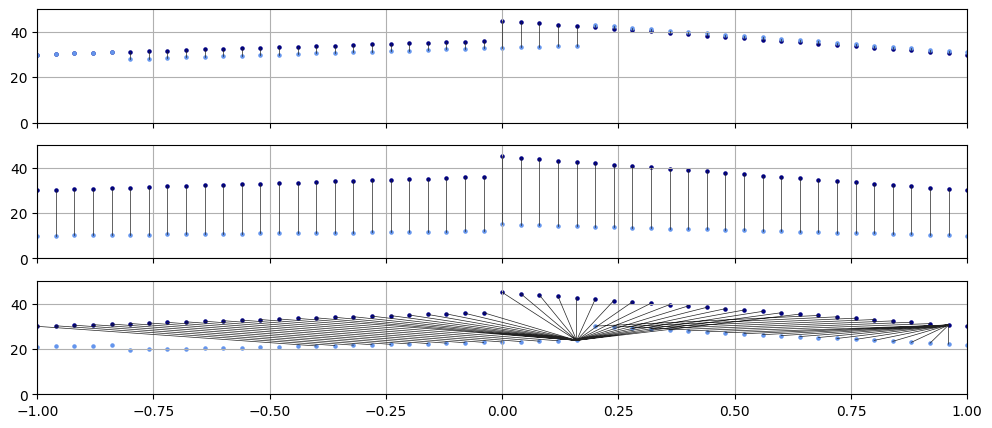
Figure 2. The ground distances between two series contributing to the overall similarity. Overlap (top panel), correlation (middle panel), DTW (bottom panel). The points between which the ground distances are calculated are represented by dark gray lines.
Results
Statistical descriptors
We are in the most fortunate position of the population being all Adele studio album songs and the sample is all Adele studio album songs. All statistical descriptors, such as mean, median etc are therefore exactly known.
Pairwise song distances
Let us describe the pairwise distances, $d_{i,j}$. They are shown in left panel of Figure 3. by tracks. They range from about 0.5 unit to 16 units. The maximum possible distance is hundred. It would be observed between two tracks where one was on the auditory limit the other was of the pain threshold throughout. We know from the previous post that the smoothed loudness does not exceed 40 units with its median being around 22 units. (Aside, the DTW distances must be unitless as they are a combination of temporal and auditory distances).
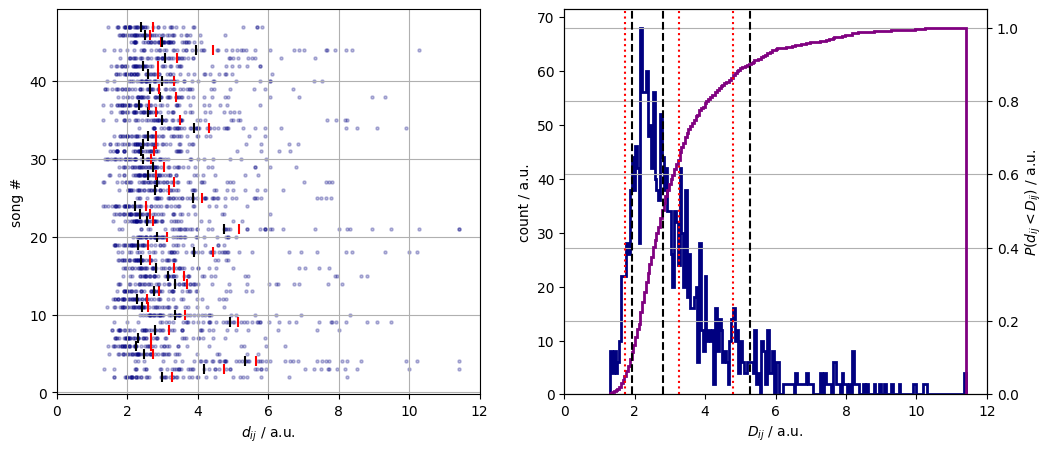
Figure 3. The song pair distances with track-wise means (red bars) and medians (black bars), (left panel). The histogram of the song pair distances, (blue line) and their cumulative distribution function (purple line), (right panel).
The mean pairwise distance, $\bar{d}_{ij}$ is 3.3. It means that any two songs is expected to be separated by about 3% loudness from the first to the last second. Strictly speaking, this is only true if the points are coupled diagonally. Given that the timepoints are separated by 1/ 1000 units, the bulk of the distance is due to auditory differences.
The queries that can be satisfied with these numbers are
- which two songs are the most similar
I miss you–Sweetest devotion
- which two songs are the least similar
Chasing pavements–Rumour has it
Average song distance
The question: how similar is a song to all the other is answered by the mean (or median) song distance:
\[\bar{d}_{i} = \frac{1}{N - 1}\sum\limits_{j=1}^{N}d_{ij}(1 - \delta_{ij}) \, ?\]This quantifier enables us to execute simple queries such as
- finding the song which is the most similar to every other
Someone like you
- identifiying the song which is the least akin to the rest.
Chasing pavements
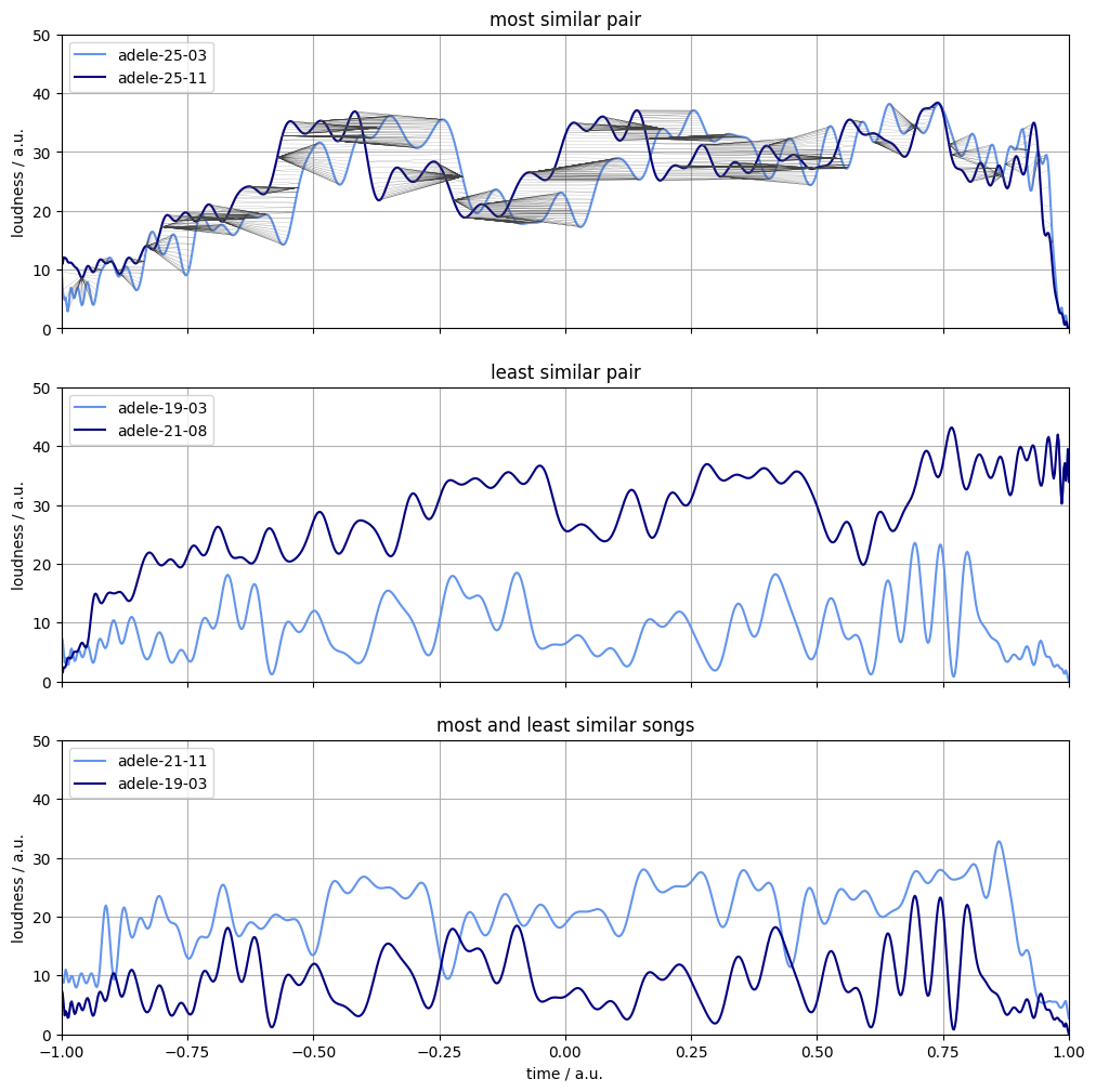
Figure 4. The most similar pair of songs (top panel), the least similar pair of songs (middle panel), the most and least alike songs on average (bottom panel). The warping path is represented by dark gray lines in the top panel.
Comparison to reference data
It is intriguiging to know whether the songs above are distinguishable from the body of pop songs. More accurately, with what degree of certainty are they more/less akin to each other than the charting songs?
Data source
Two hundred songs that charted in the UK were downloaded. Fifty from each year – 2008, 2011, 2015 and 2021 – when a studio album by Adele were released. Care was taken not to include any of her output in this sample. These lots were handled together and subjected to the exact same treatment as those by the singer scrutinised.
Distances
The DTW-s were calculated for all pairs. The raw distances and their histogram look different to those of the Adele songs. The reference pairwise distances are, on average, larger. A grand mean of 4.2 as opposed to 3.3 is observed. The mean song distances are also shifted to greater values with respect to those of the tracks of Adele.
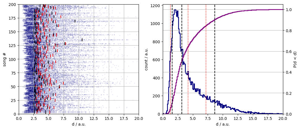
Figure 5. The song pair distances with track-wise means (red bars) and medians (black bars), (left panel). The histogram of the song pair distances, (blue line) and their cumulative distribution function (purple line), (right panel).
Statistical testing
It is almost always nearly impossible to prove whether two samples are from the same distribution as a binary answer. In order to do it, one either need to confirm that the two samples are generated by the exact same process. Alternatively, it is demanded to deduce that the two distributions are identical i.e. all moments – if defined – are equal, or they have the same characteristic function.
What is possible, on the other hand, to derive the probability of observing a quantity given
- the two distributions are identical
- the two distributions are not identical
- observing a statistical descriptor given the data and assuming a distribution
Setup
Let $\mathcal{S}$ be the set of all songs that charted in the years when the artist released an album.. $\mathcal{A}$ denotes the collection of peices by Adele. It is called the test set. Then $\mathcal{R} = \mathcal{S} \setminus \mathcal{A}$ is the reference set.
\[\begin{eqnarray} d_{ij} & = & d(s_{i}, s_{j}): s_{i}, s_{j} \in \mathcal{S} \quad & \text{(shorthand for pairwise distances)} \\ % \tilde{D}_{A} & = & \text{Median}(\{ d(s_{i}, s_{j}) : i \neq j, s_{i}, s_{j} \in \mathcal{A} \}) \quad & \text{(median of test set DTW-s)} \\ % \tilde{D}_{R} & = & \text{Median}(\{ d(s_{i}, s_{j}) : i \neq j, s_{i}, s_{j} \in \mathcal{R} \}) \quad & \text{(median of reference set DTW-s)} \\ % \end{eqnarray}\]The question is what is the probability of observing the test median if it comes from the reference distribution of the medians:
\[\begin{eqnarray} \tilde{d}_{a} & \sim & P_{A} \quad & \text{(distribution of test median)} \\ % P_{A}(\tilde{d}_{a}) & = & \begin{cases} 1 \iff \tilde{d}_{a} = \tilde{D}_{a} \\ 0 \iff \tilde{d}_{a} \neq \tilde{D}_{a} \\ \end{cases} \quad & \text{(test median is exactly known)} \\ % \tilde{d}_{r} & \sim & P_{R} \quad & \text{(distribution of reference median)} \\ % P ( \tilde{d}_{a} & \sim & P_{R} \land \tilde{d}_{a} = \tilde{D}_{a} | \tilde{d}_{r} \sim P_{R} ) \quad & \text{(test median is from the reference distribution)} \end{eqnarray}\]We are in the priviledged position of knowing the test median exactly. Sadly enough, we only have a rather flimsy estimate of the reference one. There were thousands of songs that charted in the years investigated. The entirety of them is the population. Only two hundred of them are included in our sample, $\mathcal{R}^{‘}$. Thus only a point estimate of the median is known.
Our worry is twofold:
- how representative is the sample of the population? (i.e. is it biased?)
- if it is representative, how closely can the population median be estimated?
Sample selection
Let us address the first of our concerns. The reference set is the population of all songs that reached the top hundred position in the UK in the year when a studio album was released by Adele. A sample from reference set was chosen randomly (recurrent and new Christmas singles were excluded). It is believed that the author had no bias at selecting them. The reference songs can still, nevertheless, share characteristics that set them aside from those which did not reach the top hundred. This is due to something called popular state (Zeitgeist in older literature) and is not disputed here no matter the temptation.
Bootstrapping
Even if the sample supposedly shares the required properties with the population, its small size renders any single point estimate doubtful in its validity. What if these two hundred songs constitute a subset whose median matches the test median by chance. Or, on the contrary, it is off by a long chalk?
Let us assume that the sample is representative of the population. Let us then first just randomly choose 47 songs of the 200, and calculate the median. Then estimate the median from a new selection of 47. It is likely to be different to the first one. If we repeat this procedure thousands of more times we will obtain an array of sample medians. The estimate of the reference median is the mean of those of the samples. The percentiles can also be read off from the array of values.
\[\begin{eqnarray} ! \mathcal{I} & = & [1, 2, ..., |\mathcal{S}| \quad & \text{(original sample indices)} \\ % ! N & \in & \mathbb{N}, 0 < N < \infty \quad & \text{(number of individuals in a bootstrap sample)} \\ % ! \mathcal{N} & = & [1, ..., N] \quad & \text{(bootstrap sample index set)} \\ % ! B & \in & \mathbb{N}, 0 < B < \infty \quad & \text{(number of bootstrap samples)} \\ % !n & \in & [1, ..., B] \quad & \text{($n$-th bootstrap sample)} \\ % (i_{1}, i_{2}, ..., i_{N})_{n} & = & \mathcal{B}_{n} \in \mathcal{I}^{\mathcal{N}} \quad & \text{(individuals by index in a single bootstrap sample)} \\ % \hat{\tilde{d}}_{n} & = & \text{Median}\left\{ \forall i_{k}, i_{l} \in \mathcal{B}_{n}, i_{k} \neq i_{l} : d_{i_{k}i_{l}} \right\} \quad & \text{(median of a single bootstrap sample)} \\ % \hat{\tilde{d}} & = & \frac{1}{B}\sum_{n=1}^{B}\hat{\tilde{d}}_{n} \quad & \text{(final median estimate)} \end{eqnarray}\]Note: It is not required to choose 47 songs. We can – and would be better to – select a larger number of them. The selection is by replacement, that a single song can appear in the sample multiple times.
Verdict
The bootstrapped reference set median, $\hat{\tilde{d}}{R}=3.2$, and the test median, $\tilde{d}{A} = 2.8$, are not equal. They are show in Figure 6. along with a succession of bootstrapped median distributions. Since $tilde{d}{A} < \hat{\tilde{d}}{R}$ we are interested in the probability of observing a test median less than or equal to the actual one given that it is distribution is that of the reference medians. This value can readily be obtained from the final, sixth, Figure, and it is 7%.
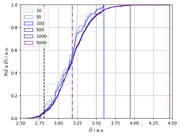
Figure 6. A sequence of bootstrap reference median distributions (pale blue tp purple solid lines). The reference median (purple dot-dashed line), the test median (black dashed line).
As a summary, it can be concluded that the Adele songs released on albums are more similar to each other that the songs charted by different artists.