This page is the first part of a doublet post where we set out to quantify the similarity of pop songs based on their perceived loudness. The present page concerns itself with the basics of sound perception. A series of transformations are introduced which recast an MP3 record to a flow of loudness.
Notes
The raw notebook is placed in this folder. It invokes the scripts which are in this repository.
Introduction
It may seem somewhat backward to entertain oneself with hand crafting features of the basest kind when online utilities are at one’s immediate disposal whereby entire albums can be created not only with voices but the styles of artists. Still, it is delightful to be reacquainted with simple notions and methods around them. Rome was not built in a day after all. This post follows a path of manipulations which takes the physical signal stored in a digital record and changes it until it represents the sensation induced by it in humans. This sensation is the loudness.
Sound in science
The ear perceives the vibrations in the medium in which it is immersed. More often than not it is air. The vibrations traverse as successive compressions and rarefactions of the medium. How quickly it changes from the thinest to the densest at a given point is the frequency. The difference between the minimum and maximum densities, roughly speaking, is the amplitude of the waves. A denser layer of particles bouncing on the eadrum at the same velocity (cf speed of sound) causes a larger movement of the membrane than if it were hit by a rarer front of particles. The stronger the push, louder the sound.
Hello sine wave, my old friend
A sound can be composed of multiple frequencies of different amplitudes. Each of them is still a wave – a succession spatial and temporal density changes. These minute variations sum up and propagate in the medium. At a fixed location, the overall density change with respect to the ambient density, or the particle displacement is given by a sum of sine waves.
\[A(t) = \sum\limits_{i=1}^{N} a_{i} \sin(\omega_{i} t + \phi_{i})\]- at a given time, $t$
- the overall amplitude, $A(t)$
- is a sum of all individual clean tones, $\omega_{i}$
- which may start at difference times, $\phi_{i}$
Any duration of sounds can thus be recorded by listing the amplitudes, frequencies and phases. A list of $(a_{i}(t), \omega_{i}, \phi_{i}$ at a given time is called a sample. The samples ought to be close enough to each other so that there are no audible gaps of silence or other artifacts. Only gasps of listening to the favourite artists.
The first figure depicts the sum of sine waves that create the song “Helllo” by Adele through interference – mostly destructive.
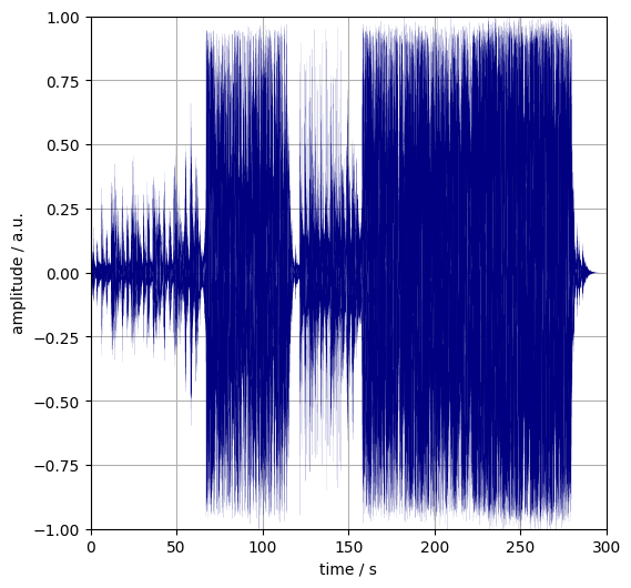
Figure 1. The waveform of the song “Hello” by Adele.
I’ve come to transform you again
The MP3 format stores the sine wave representation of a sound sequence. It does a few little tricks based on the inner workings of the human ear to reduce the file size. It is similar to the jpeg image compression algorithm in this regard. jpeg uses the psychophysical model of how sensity the eyes to certain colour combinations. MP3 considers the sensitivity to multiple concurrent frequencies.
Once the waveform is recovered from an MP3 file, it can readily be plotted. The following is observed
- the
yvalues (amplitude) ranges between$\pm 1$ - the plot looks like the audience of a sold out Taylor Swift gig attended only by hedgehogs
The latter is due to the closed spacing of the samples. The sampling frequency – or rate – needs to be at keast twice that of the highest pitch recorded in order to represent it faithfully (cf. Nyquist frequency). There are 20,500 points per second, something that we need to consider when calculating loudness.
1. A-weighting
The perceived loudness of a tone is a function of its frequency. (It is also depend on its duration and which other tones are present. Both of effects are ignored in the present discussion). The most commonly used correction is the so called A-weighting which renders the waves in the 2000–4000 Hz range lounder.
\[a_{i}^{*}(t) = f_{AW}(\omega_{i}) \cdot a_{i}(t) \quad \text{(scale amplitude according to its fequency)}\]We reweight the amplitudes of each frequency at every sampling point. The waveform_analysis package conveniently achieves this for us.
2. Amplitude to sound pressure level
The pressure differences which are processed by the listener without disabling them range over tens of orders of magnitude. It is more convenient to treat and plot their logarithms. The sound pressure level (SPL) is the logarithm of the ratio of the actual and a reference pressure.
A reference is needed because the loudness is a relative notion. Loudness also appears in relative comparisons, such as the abstract jazz band was half as loud as the audience. As a consequence, the zero of the SPL scale is not, and cannot be, fixed at absolute silece. The pivot of the scale, $p_{0}$ is the pressure change associated with quietest sound audible by the average adult human without hearing impairment. In air, it is around 20 micropascals.
\[SPL(t) = 10 \log_{10}\left( \frac{p(t)}{p_{0}} \right)\]3. Shifting
The waveforms converted to sound pressure levels range from $10^{-44}$ to $10^{+0.1}$. This corresponds to the decibel (dB) range of -440–0.1, where there reference pressure is 1 a.u.. The human ear can process about a dB range of 160 above the auditory limit. The bottom eighty of which is not painful, unless one is listening to nu-metal. We thus need to select a span of eighty. By looking at the bundled histograms of the songs in Figure 2:
- less than 0.1% of the samples is above 0 dB
- less than 1.0% of the samples is below -80 dB
Thus,
- we keep the -80 to 0 dB values of the time series and clip anything outside of this range to the nearest limit.
- set $p_{0}=10^{-4} \text{ a.u.}$, so that the lowest levels are on the auditory limit i.e. the maximum is at 80 dB.
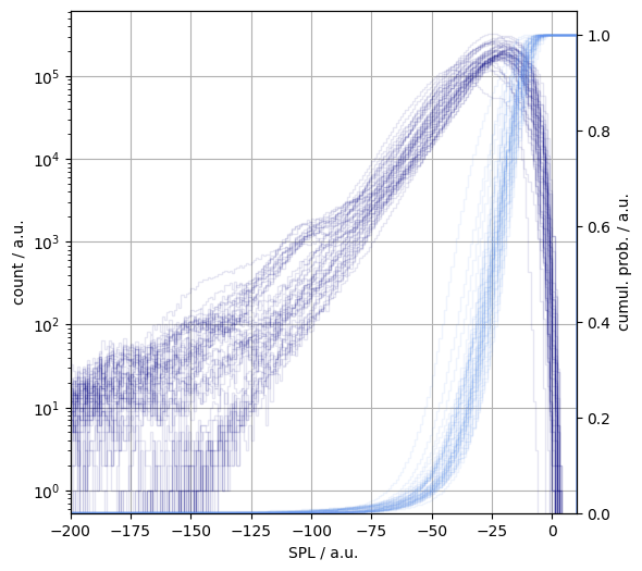
Figure 2. The sound pressure level histograms of the four investigated Adele albums. Raw counts (navy), cumulative probability function (light blue).
4. Perceived loudness
The tally of papers invesitgating the relationship between the perceived loudness and the sound pressure level greately exceeds the number of subjects on which they are based. Steven’s power law, inflected exponential function, to name two. We however proceed to use the old and trusty rule of thumb: every 10 dB increase doubles the volume, $L$:
\[L = L_{max} \cdot 2^{\frac{SPL}{10}} \, ,\]where $ L_{max}$ is the maximum of the perceived loudness. It is set at hundred.
5. Subsampling
The sampling rate is 22,050 $s^{-1}$ so that a song on average contains 4.5 milion amplitude samples. Assessment of the progression of loudness demands much fewer points. About one value in every one tenth of a second should suffice. The average loudness is calculate at every hundred millisecons. We partition the time series in a sequence of non-overlapping windows each having a span of 0.1 s. The loudness is simply the mean of the sample values in window. A random weighting is applied to the original values lest aliasing being introduced.
\[\begin{eqnarray} \hat{L}(t) = \hat {L}(i \Delta t) = \hat{L}_{i} & = & \sum\limits_{j = - \frac{m}{2}}^{\frac{m}{2}} L_{i - j} \cdot w_{j} \quad & \text{(symmetric window)} \\ % 1 & = & \sum\limits_{j = - \frac{m}{2}}^{\frac{m}{2}} w_{j} \quad & \text{(random weights)} \\ % \forall j \in [1, m]: w_{j} & \sim & \texttt{Uniform}(0, 1) \quad & \text{(uniformly distributed weights)} \end{eqnarray}\]6. Smoothing
The resultant time series is still ridden with ripples. These oscillations will add to the dissimilarity of the slower trends of the loudness. Making them smoother would accentuate contribution the overall loudness features. There are numerous methods the reduce the fast details. We elect to expand the subsampled series in terms of Legendre polynomials, $P_{k}$. Doing so is a numerically efficient way to smooth the curves – no optimisation needed.
\[\begin{eqnarray} \tilde{i} & = & \frac{i}{N} - 1 \quad & \text{(scale indices to the [-1, 1] range)} \\ % \hat{L}_{i} & \approx & \tilde{L}_{i} = \sum\limits_{k = 0}^{K} c_{k} P_{k}(\tilde{i}) \quad & \text{(expand with Legendre polynomials)} \end{eqnarray}\]The number of polynomials is set at 25. It is sufficient enough to capture the changes of the scale of iterest without introducing oscillations (Runge phenomenon).
7. Rescaling
In order to remove differences of the loudness outlines arising from the unequal lenthgs of the songs, their time points are scaled to the $[-1, 1]$ range. Two thousand equidistant samples are taken from this interval. This roughly equates the sampling frequency to $10 \text{ s}^{-1}$. The rescaling is efficiently done by reusing the Legendre expansion coefficients from the previous step. The third figure provides a graphical summary of the start and final time series and the various transforms detailed above.
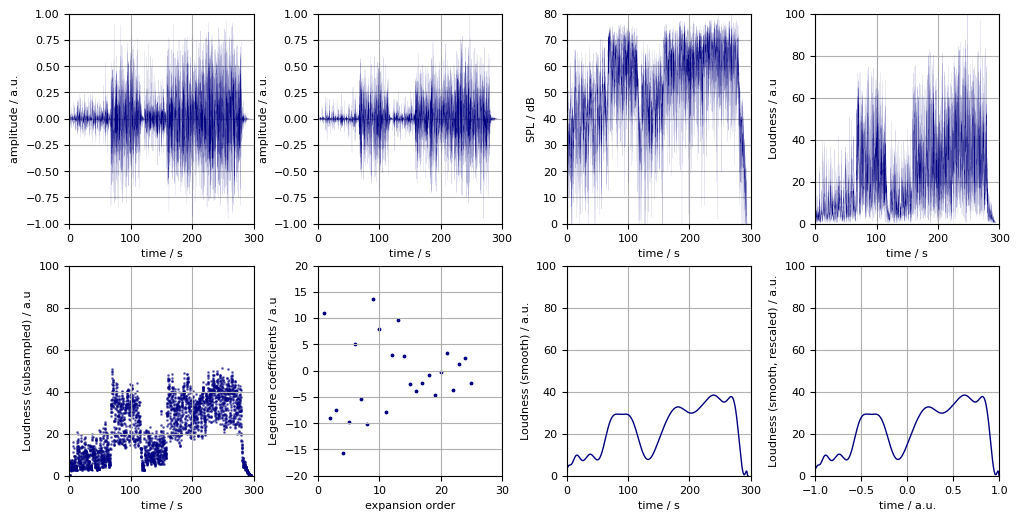
Figure 3. The original waveform of the song “Hello” by Adele (top left panel), the transforms (from left to right, top to bottom) linking it to the rescaled smoothed perceived loudness (bottom right).
Summary
We transformed waveforms stored as MP3 files to perceived loudness time series. Each of them is stored as the Legendre expansion coefficients which means a 100,000-fold reduction in size. We shall investigate how similar these loudness patterns are in the following post.
The sequence of modifications were applied to a number of albums. Four of them, with constant lyrical content throughout, are plotted in Figure 4.
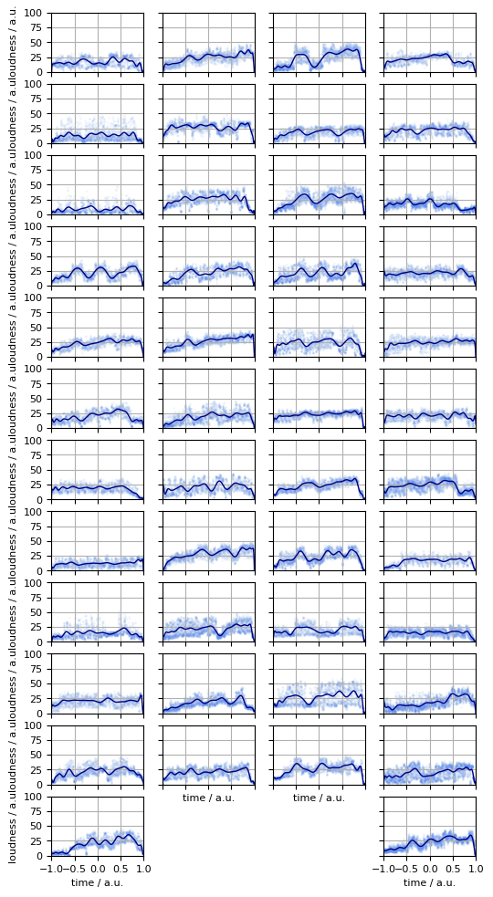
Figure 4. The perceived loudness progressions of the oeuvre of the famed singer, Adele. Legendre reconstruction (navy lines), subsamples (light blue dots).