Introduction
This short entry examines the simlarity of Formula 1 race tracks. Geometric and path based, namely dynamic time warping (DTW) and Frechet, distances are evoked to find distinct groups of tracks.
Notes
This post does not contain code snippets. The well defined units of codes were deposited in the src folder. Those were then called from the raw notebook to create this blog post.
Data
Data source
The Formula 1 track data records were downloaded from Tomislav Bacinger’s superbly curated collection and stored as json files.
Data content
Each record contains
- the name of the circuit
- the length of the circuit
- the raceline of the circuit as a sequence of geographical coordinates
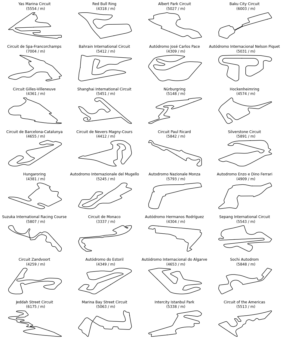
Some fields were omitted because they would not be relevant to the scope of this blog entry. The tracks with their names are displayed below. Their order remains unchanged throughout this blog post. The reader is thus kindly asked to use the figure below as a reference.
Data preparation
Centring and conversion to planar coordinates
The racelines are specified in the geographic coordinate system where each datum is a pair of longitude and latitude in degrees. There are three issues with this framework.
- They contain information about the relative positions of the circuit over the globe which is irrelevant to the similarity.
- The distances are calculated through trigonmetric formulae which is has a higher computational cost than that of the simple Euclidean distances.
- The distances are expressed in terms of arclengths as opposed to the more familiar lengths.
The coordinates of each raceline are thus centred, projected to a plane and quantified in terms of metres. The projection onto a plane inevitably leads to distortion whose magnitude can easily be estimated.
Let minimum and maximum latitudes be $\phi_{l}, \phi_{u}$. $\delta_{\lambda}$ denotes the difference of the maximum and minimum latitudes. The distance along $\phi_{l}$ is $\sin \phi_{l} R \delta_{\lambda}$ and along $\phi_{u}$ is $\sin \phi_{l} R \delta_{\lambda}$. Their ratio is
\[\alpha = \frac{\sin \phi_{l}}{\sin \phi_{u}} = \frac{\sin \phi_{l}}{\sin (\phi_{l} + \delta_{\phi})} \approx \frac{\sin \phi_{l}}{\sin (\phi_{l}) + \delta_{\phi} \cos(\delta_{\phi})} \approx \frac{\sin \phi_{l}}{\sin (\phi_{l}) + \delta_{\phi}}\]where $\delta_{\phi}$ is the span of the latitudes which is at most $~3.5\cdot 10^{-4}$ radians in the present dataset. The distortion is thus in the region of $10^{-4}$.
The conversion is performed by the function convert_lonlat_to_xy which is found in the raw notebook.
Interpolation
The reader has surely noticed gaps in the traces of the racelines in Figure 2. A track is broken down to a sequence of linear segments. The discontinuity is the missing segment betwene the last and the first points. The point between the endpoints of this section, as well as the others, can potentially carry information about about the shape of the track. An other issue is the unequal number of points. Many similarity measure demands equal number of points. The racelines are therefore interpolated. There are two obvious ways to do so
- use an identical resolution across all racelines
- use an identical number of points across all racelines
Both options are implemented in the modestly interesting function piecewise_interpolate. It will always be stated which method is used.
Similarity
Definitions
A raceline, or trace, is a twodimensional curve $\mathbf{s} \in \mathbb{R}^{n \times 2}$. The basis in which they are parametrised will change throughout this blog entry and will be specified.
Procrustes analysis
The race tracks are considered as closed curves without a sense i.e. the racecars can traverse from it any point in both directions.
Setup
The similarity is measured by the the root mean squared difference between the paired points of two traces $\mathbf{s}$ and $\mathbf{t}$.
\[\begin{eqnarray} ! \mathbf{s}, \mathbf{t} & \in & \mathbb{R}^{n \times 2} \\ d_{P} & = & \left[ \frac{1}{n}\sum\limits_{i=1}^{n} (s_{i,1} - t_{i,1})^{2} + (s_{i,2} - t_{i,2})^{2} \right]^{\frac{1}{2}} \, . \end{eqnarray}\]Rotation $\mathbf{t}$ is a rotated version $\mathbf{s}$. The Procrustes distance is the minimum $RMSD$ that can be achieved through rotations in the plane.There are number of issues with this rather naively defined distance whi are addressed below
The rotation matrix, $\mathbf{R}$ has a single parameter in two dimensions, the angle of rotation, $\alpha$:
\[\begin{eqnarray} \mathbf{R}(\alpha) & = & \begin{bmatrix} \cos \alpha & - \sin \alpha \\ \sin \alpha & \cos \alpha \end{bmatrix} \\ \mathbf{s} & \in & \mathbb{R}^{n \times 2} \\ \mathbb{R}^{n \times 2} & \ni & \mathbf{t}\mathbf{R}(\alpha) \\ t_{i} & = & s_{i} \mathbf{R}(\alpha) \, .\\ \end{eqnarray}\]Parametrisation It is the most convenient to calculate the distances in Euclidean coordinates thus the tracks are parametrised in orthogonal planar coordinates.
Interpolation In order to calculate this quantifier the compared racelines must have an equal number of points. The equal number interpolation will thus be used. Three hundred points yields resolutions between 7 metres and 24 metres.
Scaling If we are only interested in the similarities of the shapes, the racelines should be scaled to unit length to exclude dissimilarities due to their different lengths. We decide against doing so, in order keep this measure more comparable to the ones developed later on.
Reflection Two dimensional rotations cannot transform mirror images to each other if they do not have a $C_{2n}$ rotation axis. However, the shapes are deemed similar by the human eye. Therefore we allow for mirroring. The index reversing operator, $\mathcal{O}$ reverses the order of the indices
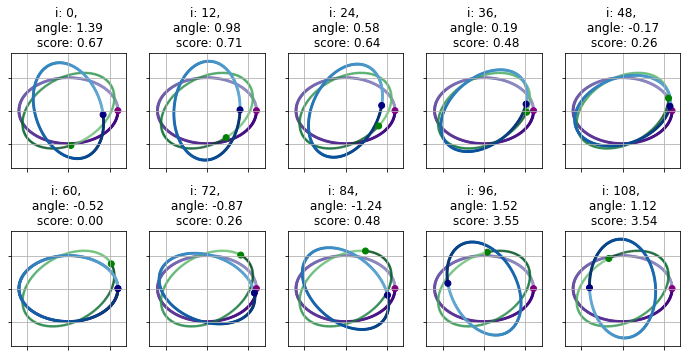
\[\begin{eqnarray} \mathcal{M}(\cdot, i) & \in & \left( \mathbb{R}^{n \times 2}, \mathbb{R}^{n \times 2} \right), i \in \left[-1, 1 \right] \\ \forall \mathbf{s} & \in & \mathbb{R}^{n \times 2}: \mathcal{M}(\mathbf{s}, i) = \mathbf{t} \in \mathbb{R}^{n \times 2} \\ t_{j} & = & \begin{cases} -s_{j, 1}, s_{j, 2} \, \text{if} \, i = -1 \\ s_{j} \, \text{if} \, i = 1 \, . \end{cases} \\ \end{eqnarray}\]Ordering – cyclic shift In addition, pairing assumes a defined and order of the points, as such the result will depend on where the numbering of the points starts in a given track. The similarities will be calculated along a medium coarse index shifting sequence to find the best matching. The shift operator $\mathcal{S}$ cyclically shifts the indices of the coordinates:
\[\begin{eqnarray} \mathcal{S}(\cdot, i) & \in & \left( \mathbb{R}^{n \times 2}, \mathbb{R}^{n \times 2} \right), i \in \left[1, ..., n \right] \\ \forall \mathbf{s} & \in & \mathbb{R}^{n \times 2}: \mathcal{S}(\mathbf{s}, i) = \mathbf{t} \in \mathbb{R}^{n \times 2} \\ t_{j} & = & \begin{cases} s_{j - i} \, \text{if} \, i < j \leq n \\ s_{n - j} \, \text{if} \, j \leq i \, . \end{cases} \\ \end{eqnarray}\]The importance or ordering is illustrated below through an example of a rotated ellipse.
Ordering – reversion of indices The overlap does depend on the relative order of the indices. Image two copies of the same shape perfectly aligned. If the points of the second one is reindex starting from the last point the overlap between the original and renumbered shapes is likely to be smaller – higher RMSD – even if the best rotation is applied due to the likely lack of symmetry. In order to mitigate this effect both the original and reversly numbered points are rotated to find the best alignment. The reflection, or mirroring operator $M$, inverts the first coordinates of the points. The index reversing operator, $\mathcal{O}$ reverses the order of the indices
\[\begin{eqnarray} \mathcal{O}(\cdot, i) & \in & \left( \mathbb{R}^{n \times 2}, \mathbb{R}^{n \times 2} \right), i \in \{ -1, 1 \} \\ \forall \mathbf{s} & \in & \mathbb{R}^{n \times 2}: \mathcal{O}(\mathbf{s}, i) = \mathbf{t} \in \mathbb{R}^{n \times 2} \\ t_{j} & = & \begin{cases} s_{j} \, \text{if} \, i = 1 \\ s_{n + 1 - j} \, \text{if} \, i = -1 \, . \end{cases} \\ \end{eqnarray}\]Algorithm
Each track is represented by the same number of coordinates which are centred. It finds those parametrisations of operator the actions of whose of a set of track coordinates minimises the RMSD with respect to an other set of track coordinates.
\[d_{P}^{*} = \min \{ d_{P} \left( (\mathcal{R}(\alpha) \mathcal{M}(i) \mathcal{S}{j} \mathcal{O}(k)\mathbf{s}), \mathbf{t} \right), \, {\alpha \in [0, 2 \pi ), \, i \in [-1, 1], \, j \in [-1, 1] , \, k \in [-1, 1]} \}\]The minimisation algoritm does not extend beyond a few lines of the calc_dist_proc function.
Dynamic time warping
The race tracks have so far been treated as closed curves without a defined direction along which they are traversed. This is however not the case. They have a defined starting point and a strictly enforced sense in which they must be traversed. These requirements redefine the tracks as a sequence of features, such as straight lines, left turns, right turns of various curvature. A quantifier that tries to match these features in order is thus gives us a more realistic measure of similarity. Once such measure is the dynamic time warping (DTW).
It is instructive to think about the DTW as a minimum length path in the directed graph of the pairwise distances. For two tracks $\mathbf{u}$ and $\mathbf{v}$ the graph $G = (V, E)$ is defined as follows: \(\begin{eqnarray} \mathbf{u} & \in & \mathbb{R}^{n}, \mathbf{v} \in \mathbb{R}^{m} \\ V & = & \{ (u_{i}, v_{j}): i \in \left[1, ..., n \right], j \in \left[1, ..., m \right] E \subset V \times V \\ \forall \, (e_{i}, e_{j}) & = & ((u_{k_{i}}, v_{l_{i}}), (u_{k_{j}}, v_{l_{j}})) \in E: \\ k_{i} & = & k_{j} \land l_{i} + 1 = l_{j} \\ \lor \\ l_{i} & = & l_{j} \land k_{i} + 1 = k_{j} \\ \lor\\ k_{i} + 1 & = & k_{j} \land l_{i} + 1 = l_{j} \end{eqnarray}\)
All edges can only point left, down or diagonally down. As such, $(V, E)$ is a directed graph. As a consequence, a weight can be assigned to each edge using its target vertex. The weight of an edge is the distance between the points defining its target:
\[\begin{eqnarray} e & = & ((u_{k_{i}}, v_{l_{i}}), (u_{k_{j}}, v_{l_{j}})) \\ w(e) & = & d(u_{k_{j}}, v_{l_{j}}) = d_{k_{j}, l_{j}} \, . \end{eqnarray}\]The dynamic time warping distance is then the minimum path between $(u_{1}, v_{1})$ and $u_{n}, v_{m}$.
\[\begin{eqnarray} r & \in & [m + (m - n) - 2 , m + n - 2] \\ p & \in & E^{r}: \\ p_{1, 1} & = & (u_{1}, v_{1}), p_{r,2} = (u_{n}, v_{m}), \\ \forall i & \in & [1 - r-1]: p_{i, 2} = p_{i+1, 1} \\ \mathcal{P} \\ d_{DTW}(\mathbf{u}, \mathbf{w}) & = & \min_{p \in \mathcal{P}} \big\{ \sum\limits_{e \in p} w(e) \big\} \\ & = & \min_{p \in \mathcal{P}}\big\{ \sum\limits_{(k_{i}, l_{i}) \in p} d_{k_{i}, l_{i}} \big\} \\ & = & \min_{p \in \mathcal{P}}\big\{ \big[ \sum\limits\limits_{(k_{i}, l_{i}) \in p} |d_{k_{i}, l_{i}}|^{1} \big]^{\frac{1}{1}} \big\} \end{eqnarray}\]Frechet distance
The last term was written as a sum of the modulus of the distances under the first root. It may seem superflous, but it provides a way to link the DTW distance to the Frechet distance, $d_{F}$. The latter one is the minimum length path between the same two points where the distance is the maximum edge weight encountered along the path.
\[\begin{eqnarray} d_{F}(\mathbf{u}, \mathbf{w}) & = & \\ & = & \min \{ \max \{ w(e_{i})\, \, e_{i} \in p\} \, p \in \mathcal{P} \}\\ & = & \min_{p \in \mathcal{P}}\big\{ \sum\limits_{e \in p} w(e) \big\} \\ & = & \min_{p \in \mathcal{P}}\big\{ \big[ \sum\limits\limits_{(k_{i}, l_{i}) \in p} \lim_{q \rightarrow \infty} \big[ \sum\limits_{i=1}^{r} |d_{k_{i}, l_{i}}|^{q} \big]^{\frac{1}{q}} \big\} \end{eqnarray}\]Aligning the tracks
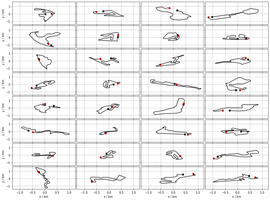
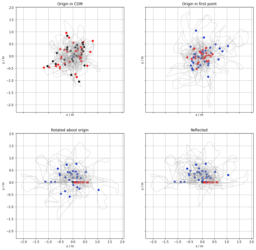
The origin of a raceline coordinates was in the the centre-of-mass. This is constructive is the overall geometric shapes are compared. Shoul one wish to compare how the lines evolve along their courses they need to be aligned more carefully.
- Firstly, the origin is in the first point of track
- The first segments of the tracks are parallel (oriented in the same way)
- the bulk COM of the trace must have a nonzero oordinate. To achive this, some of the racelines are reflected with respect to the line on which the first segment lies.
The figure below shows this sequence of transformations. Again, the first and last points are emphasised by black and red dots, respectively. The centre of mass of each track is marked by a blue dot.
Calculating the path-based distances.
The calc_dtw_distance and calc_frechet_distance functions calculate the two path based distances of each pair of tracks. These functions are implemented with numba to decrease the their execution time (about 200 times speed up).
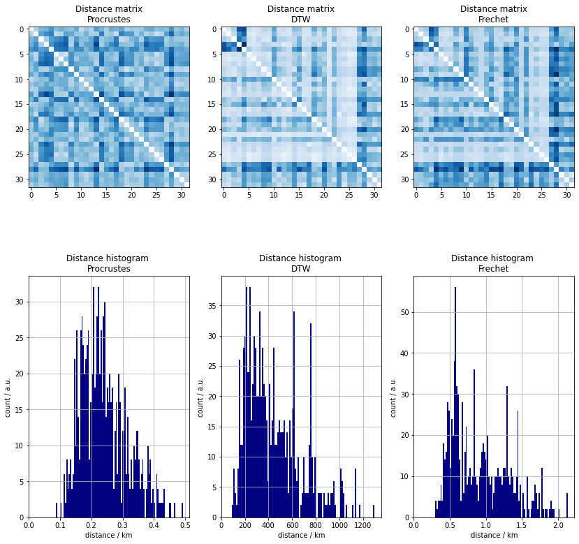
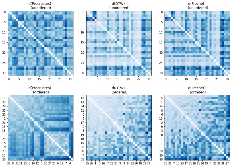
Comparison of the raw distances
The raw distances are laid out below. Each column or row represents the distances between a certain track and the others. A few observation can readily be made.
- there are tracks that are similar to each other
- the are pairs which are vastly different
- both can happen in the same row
- there are rows which tend to have lower distances than other rows. It means that certain tracks are similar to most the the other ones.
- the opposite can also happen
- there are chance rectangles where the similarity is high which implies the presence of groups of tracks that have an ovarall alike shape.
The histograms, on the other hand, do not have a distinct peak a low distances and secondary ones at larger dissimilarities which would be indicative of clusters.
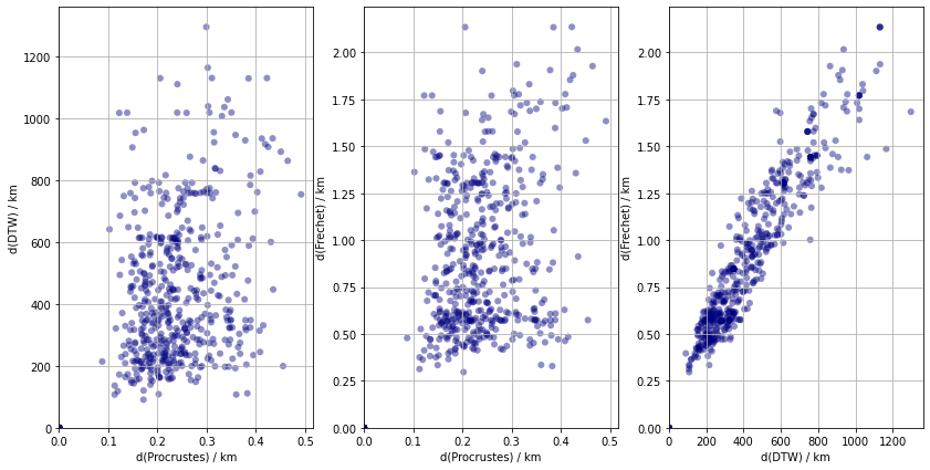
As an aside, the distributions of the two path based distances are similar apart from a scale factor. It is thus expected that a two types of similarity measures would return different possible clusters.
Analysis of the Distance Matrix
Querying the distance matrix
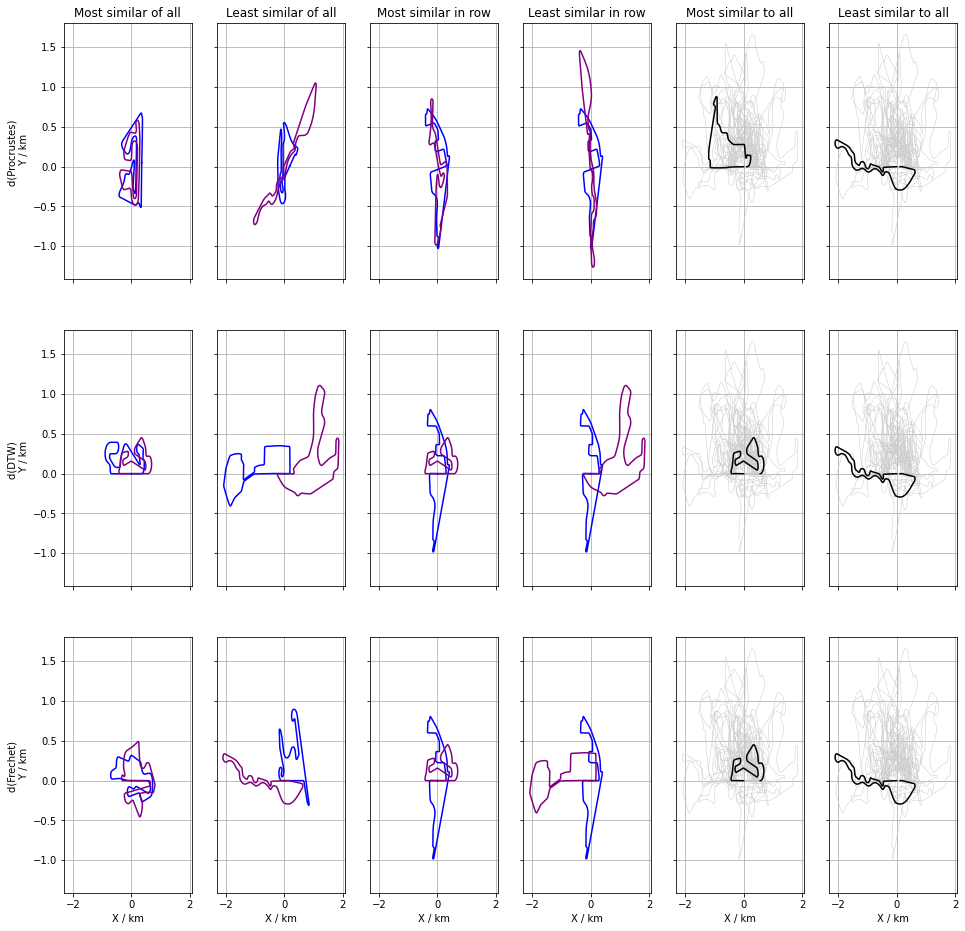
Once the distances are know, simple inqueries about the objects can be with ease. These questions are most suitable directed at relationships between pairs of objects, such a which are the two most similar track, or which resemble each other the least. The answers are given by indices of the smallest and largest distances respectively which can be found in $\mathcal{O}(N^{2})$ time.
Similarly, the indices smallest and largest element of a row belongs to the most and least similar pair where the reference is given by th row index which is an operation of a cost $\mathcal{O}(n)$. Higher order relationships, such as the three or four most similar tracks can still be found in polynomial time $O(n^{k})$ provided $k « n$ or $k \approx n$, otherwise it is an exponential problem. In either case, some of these pairwise relaionships are plotted in the next figure.
We proceed to uncover the higher order relationships with a few simple heuristics in the following.
High order relatioships – groupings
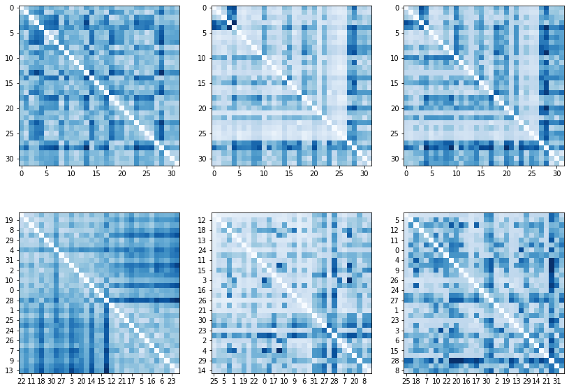
Quick clustering by vertex ordering
A grid of the overlaid racecourses along with the RMSD scores are plotted the (rather large) figure separately. Owing to the author’s mild monomania, they will be cluster in the second section of this blog post. For now, a quick and dirty cluster analysis is performed by reordering the ordering in which the courses appear in the distance matrix.
Algorithm
The minimum bandwidth form of a matrix groups sets of vertices together whose in-set pairwise distances are small compared to those between them and the elements outside of the set. The RCM, GPS and GK algorithms work of sparse matrices. We thus either threshold the RMSD values:
\[\begin{eqnarray} \mathbf{D} & \in & \mathbb{R}^{n \times n} \\ \delta & \in & \mathbb{R}^{+} \\ \mathbf{D}^{'} & \in & \mathbb{R}^{n \times n} \\ d_{ij}^{'} & = & \begin{cases} 1 \, \text{if} \, d_{ij} \leq \delta \\ 0 \, \text{if} \, d_{ij} > \delta \end{cases} \end{eqnarray}\]to create a binary matrix. In this case, the threshold must be selected, for instance, by Otsu’s method. However, it will always be arbitrary and the clusters will depend on it. Alternatively, an order similar to the minimum vertex order can easily be established, whereby the next index is those which minimises the distance to the already ordered points. The starting index can is of the most central point.
\[%\begin{eqnarray} \begin{aligned} \hline &\textbf{Algorithm 2.} \, \text{Order vertices} &\\ \hline &\textbf{Inputs} & \\ & \quad \mathbf{D} \in \mathbb{R}^{n \times n} \quad \text{(distance matrix)} & \\ &\textbf{Output} \quad \text{(index order)} & \\ & \quad \mathbf{o} \in \mathbb{N}^{n} & \\ & \mathcal{I} \leftarrow [1, ..., n] & \\ & \mathbf{d} \leftarrow \mathbf{D} \cdot \{1 \}^{n} & \\ & \mathbf{o} \leftarrow \{0 \}^{n} & \\ & i \leftarrow 1 & \\ & o_{i} \leftarrow \arg \min\limits_{j \in \mathcal{I}} d_{j} & \\ & \textbf{while} \, |\mathcal{I}| \neq 1 & \\ & \quad \mathcal{I} \leftarrow \mathcal{I} \setminus \{o_{i}\} & \\ & \quad j = \arg \min\limits_{j \in \mathcal{I}} \sum\limits_{k \in [1, ..., i]} d_{o_{k},j} & \\ & \quad i \leftarrow i + 1 & \\ & \quad o_{i} \leftarrow j & \end{aligned} %\end{eqnarray}\]There are a strong and a weak cluster which appear as blocks on centred on the diagonal. The Procrustes distances generate better defined clusters because the pairs of tracks are aligned more closely before the distance is calculated, such as rotation, reflection, alignment through shifting and reflecting indices. The graph based similarity measures, on the other hand operate on the much less aligned pairs of coordinate sequences.
This crude clustering method reminds us of Prim’s algorithm to find a minimum spanning tree of a complete graph. If that algorithm is launched from the most the same vertex i.e. the track which has the minimum pairwise distance, and a breadth first search is used to order the vertices from the same starting point, plots akin to the ones above are observed.
Displaying groups in 2D
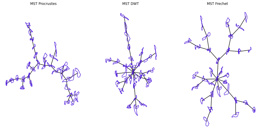
Minimum spanning tree
A simple way to visualise cluster in the plane might be through their minimum spanning trees. There are, however, three issues with this method
- the minimum spanning three does not necessarily retain clusters especially when the number of vertices are small
- the drawn segments must be proportional to the distances that they represent
- the algorithm used to plot the tree may further distort the distances between vertices because it only preserves path lengths that are in the tree
Indeed, there are edge crossing, unreasonably linear sequences of vertices tally up with our previous observations.
Multidimensional scaling
Multidimensional scaling (MDS) – roughly speaking tries to places objects in a low dimensional place in a way that their original high dimensional distances are the best preserved. There are many flavours DMS (classical, metrix, non-metric, various definitions of “distance” and quantification of being “best preserved”). In short, MDS tends to place objects close to each other which are so with respect to their original distances. The reverse is not necessarily true. Proximity of the objects in the low dimensional place does not imply closeness in the original space.
However, there are a few issues with MDS per se
- it returns solutions in an affine space, that is to compare various projections, translation, rotation and reflection may need to be applied.
Issues of implementation in
sklearn - it is not possible to scale multiple distance matrices in the same time to avoid the issue above
- it uses SMACOF which is a local optimiser
- seeded randomly which results in different projections from different runs even when the same distance matrix is treated.
Topological mapping
This term refers to methods whereby the proximity between objects is represented by edges in a graph. If the graph is planar the resulting mapping can be displayed in two dimensions. Examples are the various self organising maps, such as SOM, a growing neural gases. We will not invoke these methods in this blog post.