Analysis of UK pub names

Introduction

This post entertaines the reader to a brief analysis of the public house names in the United Kingdom. It comprises three parts. The first one executes a sequence of steps to clean a data set. Some statistical descriptors are then applied to the pub names. Finally, one of the most fundamental questions of the British life is answered: how far does one need to walk from a pub to the nearest one?

Note

The raw notebook contains the scripts that are sufficient to reproduce the workflow of these notes. It is deposited here.

Data

Source

The data was sourced from the getthedata webpage. The 02/2022 data set is investigated below.

Preparation

The table is first loaded. (It is recommended to use symbolic links to point at files.)

df_coords = pd.read_csv("path_data", header=None)

Trimming

Only the columns containing the names of the watering holes and their coordinates are retained. The columns are also renamed to reflect their content.

df_work = df_coords.copy()
df_work.drop(columns=df_work.columns[[0, 2, 3, 4, 5, 8]], inplace=True)
df_work.rename(columns={1: "name", 6: "latitude", 7: "longitude"}, inplace=True)

print(f"Number of establishments: {len(df_work)}.")

Number of establishments: 51331.

Cleaning

Corrupted coordinates

The table is riden with corrupted rows where the coordinates are missing. These are removed. A value in the latitude and longitude lists is accepted if it is parsable to a number float.

mask = (
    df_work["latitude"].apply(is_parsable_to_float)
    & df_work["longitude"].apply(is_parsable_to_float)
)
df_work = df_work.loc[mask]

# parse to float
df_work["latitude"] = df_work["latitude"].apply(float)
df_work["longitude"] = df_work["longitude"].apply(float)

print(f"Number of establishments: {len(df_work)}.")

Number of establishments: 50564.

Sanitising of the names

The ampersand & is substituted to literal and to make the coordinating conjuction consistent.
Any terminal whitespaces are removed.
Those are in medial position are replaced by a single space.
The terminal , The are removed and the remaining string is prefixed by The .
The names are also cast in title case where all letters are lowercase except for the starting letters of the words which are uppercase.

The sanitise_name function performs all these tasks.

def sanitise_name(string: str) -> str:
    """
    Sanitise names
        * remove terminal whitespaces
        * replace medial whitespaces with a single space
        * replace `&` with `and`
        * remove ", The" and add "The" as prefix
        * rewrite as titlecase
        
    Parameters:
        string: str : raw name
    
    Returns:
        string_sanitised: str : sanitised name
    """
    
    # 1) remove terminal whitespaces
    string_sanitised = string.strip().lower()
    
    # 2) replace medial whitespace
    string_sanitised = re.sub("\s+", " ", string_sanitised)
    
    # 3) replace ampersand with "and"
    string_sanitised = string_sanitised.replace("&", "and")
    
    # 4) remove suffix ", the" and prefix with "the "
    if string_sanitised.endswith(", the"):
        string_sanitised = "the " + string_sanitised[-5]
    
    # 4) titlecase
    string_sanitised = string_sanitised.title()
    
    return string_sanitised

df_work["name"] = df_work["name"].apply(sanitise_name)

Redundant suffixes

Some names end with Public House, Micro Pub, Pub, PH, P H. These can be removed without the possbility of generating erroneous entries when it is not the integral part of the name e.g. The White Lion Public House. If it is an inherent part of the name, such as the superbly original Ye Olde Public House, its removal yields an incomplete name: Ye Olde.

There are thus two options:

a name appears with and without suffix: in this case it is assumed that the bare name is a valid pub name
a name only appears with a suffix: in this case the unsuffixed name is considered a valid pub name, no matter whether it is a complete phrase of not.

The function remove_suffix deletes a specified set of suffixes from a name.

def remove_suffix(
        string: str,
        suffixes: List[str]
    ) -> str:
    """
    Parameters:
        string: str : name
        suffixes: List[str] : suffixes to remove
    Returns:
        truncated: str : cleaned string
    """
    
    truncated = string
    for suffix in suffixes:
        truncated = truncated.removesuffix(suffix)
    
    return truncated

suffixes = [
    " Public House", " Micro Pub", " Pub", "Ph", "P H"
]

df_work["name"] = df_work["name"].apply(remove_suffix, args=(suffixes,))

Irregular names

A number of names have the syntax <string-1> at <string-2>, where <string-1> is either a regular pub name or an other string. <string-2> is either a location name or a pub name. There are about 230 such entries.

Discarding the ones which refer to non-pubs and extracting those belonging to pubs are tasks to be automated. It requires crafting a classifier which flags up strings which are pub names. Given the low number of entries, as opposed to writing a utitlity, these chores were performed manually. The starting data set was already cleaned in this particular regard.

Corrupted names

A name is considered corrupted if

Its length is less than three.
Its contains non-alphabetic characters. Sorry, no hipster pubs with curly brackets.

Non-pub entries

A name is conidered to be that of a pub if

It does not end with certain words, such as centre, club, hall, ltd. etc.
Nor does it contain the words bar, pizza, association, sport etc.

This policy might be overly restrictive and result in excluding entries which indeed point at public houses. These filters, however, remove non-pubs at a higher rate than pubs. I.e. it is more likely that a location which is not classified as a public house in its common meaning have a name ending in “club” than a pub. Also, the distorting effect of a faux pub on the analysis is more significant than inaccuracies introduced by omitting proper pubs.

The function is_valid_name removes those entries whose names are deemed as corrupted or referring to non-pubs.

def is_valid_name(
        string: str,
        tokens_suffix: List[str],
        tokens_infix: List[str]
    ) -> bool:
    """
    Decides whether a string is a valid pub name.
    
    Parameters:
        string: str : possibly suffixed string
        tokens_suffix: List[str] : excluded endings
        tokens_infix: List[str] : excluded anywhere in the name
    """
    
    # corrupted name
    if len(string) < 3:
        return False
    
    # only letters
    if not string.replace(" ", "").isalpha():
        return False
    
    # lower case for a reduced number of comparison
    string_ = string.lower()
    if any(string_.endswith(token) for token in tokens_suffix):
        return False
    
    if any(string_.find(token) > -1 for token in tokens_infix):
        return False
    
    return True

Note, a little bit more could have been exercised when excluding names of chains e.g. wetherspoon. A procedure whereby the chain token is first excised from the string which is then checked for validity would have retained names compounded of chain and pub names e.g. The Pink Elephant Wetherspoon,

# exclude entries with corrupted names or those which are likely to belong to non-pubs
df_work["name"] = df_work["name"].apply(lambda x: x.title().strip())

tokens_suffix = [
    "assoc", "assoc.", "association", "buzz bingo", "casino", "club",
    " c", "centre", "fc", "hall", "hotel", "ground",
    "legion", "lounge", "park", 
    "rfc", "rlfc", "royal british legion", "rufc",
    "society", "social", "student union",
    "students union", "wine", "wmc"
]

tokens_infix = [
    " bar", "be at one", "bbq", "cafe",
     "carvery", "catering", "churcs", "coffee",
    "community", "cuisine", "club",
    "fitness", "gym", "hotel", "institute",
    "jamies", " kitchen",
    "ltd", "ltd.", "limited", "old home", "pizza", 
    "pizzeria", "prezzo", "revolution", "school",
    "slug and lettuce", " sport", "sports"
    "restaurant", "theatre", "university", 
    "walkabout", "welfare", "wetherspoon"
]

mask = df_work["name"].apply(
    is_valid_name, args=(tokens_suffix, tokens_infix)
)
df_work = df_work.loc[mask]

print(f"Number of establishments: {len(df_work)}.")

Number of establishments: 31040.

Prefixed pub names

For the purposes of this analysis, names with and without the prefix The are considered identical. We quickly scan the corresponding column for these pairs. The article is then removed from the unified name to save precious rendering time.

There are many ways to perform this task. In order to preserve the original order of the names and perform the replacement in $\mathcal{O}(N)$ time, an $\mathcal{O}(N)$ storage is needed. Lookup in a linked list is $\mathcal{O}(N)$, therefore a set of the names is created to speed up the search ($\mathcal{O}(1)$).

def create_prefix_mapping(
        strings: Iterable[str],
        prefix: str
    ) -> Dict[str, str]:
    """
    Creates a prefixed-string--string mapping from a list of strings.
    pairs: <prefix><string>: <string>
    
    Parameters:
        strings: Iterable[str] : strings which may have a prefix
        prefix: str : prefix!
        
    Returns:
        mapping: Dict[str, str] : prefixed string -- string mapping
        
    Note:
        It is wasteful to save the non-prefixed strings, however, this
        format is required in the subsequent use.
    """
    
    string_set = set(strings)
    
    mapping = {}
    
    i_bare = len(prefix)
    
    for string in strings:
        # find the ones with prefix
        if string.startswith(prefix):
            # remove prefix to get a stem
            string_ = string[i_bare:]
            
            # if the stem appears in the set on its own
            # add the pair to the mapping
            if (string_ in string_set) and (string not in mapping):
                mapping.update({string: string_})
                
    return mapping

mapping = create_prefix_mapping(df_work["name"], "The ")
df_work["name"].replace(mapping, inplace=True)

Duplicate coordinates

The coordinates are then checked for duplicates. A pub is identified by its coordinates and name. We keep only one entry per pub.

df_work.drop_duplicates(
    subset=["name", "latitude", "longitude"], keep="first", inplace=True
)
print(f"Number of establishments: {len(df_work)}.")

Number of establishments: 30995.

If there are multiple names at a location we pick one entry randomly. This is to avoid biasing towards which alphabetically preceed the others in the group should they be ordered so. Cross referencing a map from the year would help identify which entries to keep. The possible reasons of having duplicate or near duplicate coordinates are discussed in the spatial analysis section.

groups = df_work.groupby(by=["latitude", "longitude"])

# keep only groups of identical coordinates
groups = (g for _, g in groups if len(g) > 1)

idcs_to_drop = []
for g in groups:
    
    # keep only one index selected randomly
    idcs_to_drop_ = list(g.index)
    idx_keep = np.random.choice(len(g))
    del idcs_to_drop_[idx_keep]

    idcs_to_drop.extend(idcs_to_drop_)
    
df_work.drop(labels=idcs_to_drop, axis=0, inplace=True)

print(f"Number of establishments: {len(df_work)}.")

Number of establishments: 29846.

We are left with just shy of thirty thousand pubs which will be subjected to analysis.

Data analysis

Statistics on names

Let us recognise for the millionth time that pubs are christened Red Lion the most frequently in the United Kingdom.

Name propensity

Thirty thousand pubs share roughly fifteen thousand names. The eighty most popular are listed with their number of occurence in Figure 1. Indeed, the largest pride of the British pubs is that of the Red Lions.

df_propensity = df_work["name"].value_counts()
print(f"Number of names: {len(df_propensity)}")

Number of names: 14910

png

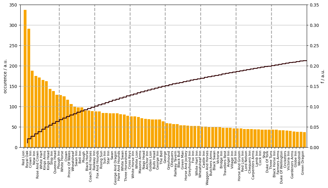
Figure 1. The occurences of the eighty most frequent pub names (golden ale bars). The cumulative distribution function of the entire set (stout line).

Name inequality

Figure 1. also shows the proportion of pubs that share the same name arranged in decreasing name propensity. For example, 10% of the pubs are baptised as one of the twenty most popular names.

To gauge the inequality of the name distribution, let us consider the most and least equal of all hypothetical scenarios:

most equal: $N$ pubs with $N$ unique names. In general, there are equal numbers of differently called pubs.
least equal: $N$ pubs with two names where one name occurs $N-1$ times, the other only once.

The equivalent allocation of $M$ names among $N$ pubs $(M \leq N)$ is the

most equal: $N = M \dot a + q, a, q \in \mathbb{N}$. If $q=0$, then $\frac{N}{M}$ pubs of each name. Otherwise, eahc name is assigned to pubs in a manner that makes the resultant distribution of the names the most similar to the uniform. “Closest” refers to attaining a value of a quantifier which the closest to the quantifier value of a uniform distribution of $M$ elements. It is usually: each of $q$ names appear $(a + 1)$ times, and $M - q$ $a$ times.
least equal: $M - 1$ names appear only once, one name is found $N - (M - 1)$ times

There is a pubload of mathematical constructs to quantify inequality. Only one of them is chosen here, the Gini coefficient. No entropy today.

For the discussion below, the names form a population totaling $M$. The wealth is the number of pubs, $N$.

Gini coefficient

The Gini coefficient is derived from the Lorenz curve which plots the cumulative wealth as a function of the fraction of population in increasing wealth. That is to say, first the names which have one pub then those with two public houses until we arrive at the Red Lion. Half of the area between the so-created curve and the one spanning between (0, 0) and (1, 1) is the Gini coefficient. If each name appeared only once the Lorenz curve would be the diagonal. The most inequal distribution would lead to a trace similar reversed L.

One formula speaks for thousand words. Two or more leave us speechless:

\[\begin{eqnarray} \mathcal{I} & = & [1, M] \quad & \text{(pub names)} \\ % \forall i & \in & \mathcal{I}: \mathbb{N} \ni m_{i} \geq 1 \quad & \text{(number of pubs with the same name)} \\ % \forall i, j & \in & \mathcal{I} : i \leq j \iff m_{i} \leq m_{j} \quad & \text{(they are ordered in ascending frequency)} \\ % x_{i} & = & \frac{i}{M} \quad & \text{(cumulative population fraction)} \\ % y_{i} & = & \frac{1}{\sum\limits_{i=1}^{M}m_{i}} \sum\limits_{i}^{m}m_{i} \quad & \text{(cumulative wealth fraction)} \\ % L & = & \{ (x_{i}, y_{i}): \forall i \in \mathcal{I} \} \quad & \text{(Lorenz curve)} % \end{eqnarray}\]

The Lorenz curve of the pub name distribution along that of the hypothetically most equal scenario are plotted in Figure 2. The Gini coefficient comes to be around 0.36 indicating medium inequality.

png

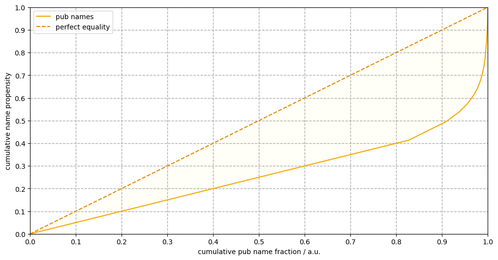
Figure 2. The Lorenz curve of the pub name distribution (golden ale line) and that of a uniform distribution (amber ale line). The half of the ratio of the head coloured area and the are of the triangle is the Gini coefficient.

The Lorenz curve is composed of two distinct ranges. The linear segment from the origin to the $x$-value of about 0.83 is spanned by the names which occur only once. To frame this positively, 43% of the UK pubs have a unique name which amounts about 83% of all individual names. This linear line is followed by a sequence of segments which sharply curves upwards. It belongs to names which are associated with more than one public houses. The last segment ends at the Red Lion.

Spatial analysis

Problem statement

We seek to answer a single question only: how long need one walk between pubs? Well, it is always the longest after the penultimate pint. In terms of distances, the query should be refined. We mean the median length of the shortest line to the nearest watering hole from any given pub.

Data structure

The naive solution is quadratic with respect to the number of pubs. That is, for each pub the distance to every other pub needs to be calculated. Obviously, we will use a data structure which cuts the time down to $\mathcal{O}(N \log N)$, where $N$ is the number of pubs. The structure of choice is the ball tree.

Great circle distance

The distance between two points on the surface of a sphere is given by the length of the arc drawn between them whose associated radius originates from the centre of the sphere. This is also known as the great circle distance. It is the shortest path between two points on a sphere.

Why cannot kD trees be used?

The python implementation of the kD-tree can only return valid query results if the distances are defined on Cartesian-like coordinates. This means that an unit change along a coordinate alters the distance along that coordidate by the same amount independently of the (constant) values of the other coordinates. This is not the case when distance is computed from latitude and longitude using the square root formula. In small areas and away from the poles the two angles behave as Cartesian coordinates. Across the entire UK, this certainly does not hold.

On option would be to convert the polar coordinates to Cartesian ones and create a tree in three dimensions. This would partition the space consistently. The underlying distance, however, would still be the Euclidean which approximates the great circle distances only in areas of small extent.

Ball tree with haversine distance

The python implementation of the ball tree. It can partition the space correctly with haversine distance. Returns the great circle distance below between points $(\phi_{i}, \lambda_{i})$ and $(\phi_{j}, \lambda_{j})$ on the unit shpere:

\[\begin{eqnarray} d_{ij}& = & 2 \arcsin \left({\sqrt {\frac {1-\cos \left(\phi _{j}-\phi _{i}\right)+\cos \phi _{i}\cdot \cos \phi _{j}\cdot \left(1-\cos \left(\lambda _{j}-\lambda _{i}\right)\right)}{2}}}\right) \, . \end{eqnarray}\]

The maximum error arising from treating the Earth as a sphere is about 0.5%. It is considerably smaller when a region of the size of the UK is investigated only.

Spatial distribution

Firts of all, let us visualise the raw coordinates. The amber ale coloured dots are absent north of the Glagow–Aberdeen axis. The advancement of the temperance movement in those regions has not made it to the news in the recent years. It is therefore assumed that the database is incomplete this area. Given the size of the population and its low density (I do hope no offence is taken Thurso or in Lerwick), the partial hiatus of the Scottish public houses do not distort our statistical findings about the names. The geospatial analysis, of course, affected. Statements about pub names in low density areas are likely to be lacking in correctness.

png

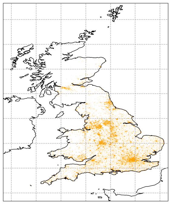
Figure 3. The spatial distribution of the pubs (amber ale dots).

Nearest neighbour distances

The coordinates are converted to radians and a ball tree is constructed from them.

df_work["latitude"] = np.radians(df_work["latitude"])
df_work["longitude"] = np.radians(df_work["longitude"])

X = df_work[["latitude", "longitude"]].values

tree = BallTree(X, metric="haversine")

Since the duplicate coordinates were removed, it is safe to perform a spatial query for two pubs closest to the each pub. The second least distant will be the true nearest neigbour on the globe.

dists, idcs = tree.query(X, k=2)
dists = dists[:, 1] * RADIUS_EARTH
idcs = idcs[:, 1]

The distribution of the nearest neighbour distances are plotted on a logarithmic abscissa in Figure 3.

png

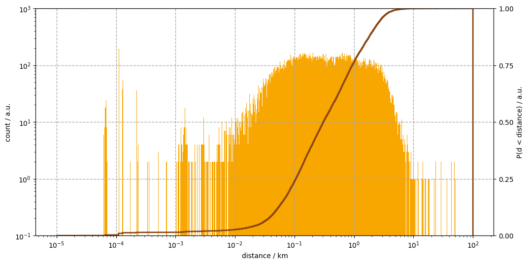
Figure 4. The occurences of the eighty most frequent pub names (golden ale bars). The cumulative distribution function of the entire set (stout line).

The first feature to notice is the cluster at $10^{-4}\text{ km} = 10 \text{ cm}$. A brief investigation which can be found in the raw notebook, reveals that these are mostly not due to pubs of variant names e.g. “Red Lion” and “Red Lion Inn”. It most likely stem from erroneous coordinates or recording both the old and the newer names of the same establishment.

The coglomeration of distances in the range of few ten metres represents presumably entries of inaccurate locations and real clusters of pubs (the author was able to recall instances of both from memory). Cross-referencing the database with current maps the most surely resolve these and other previous issues.

The first two details only ammount for less than two percent of all distances. The bulk of the distribution spreads across three orders of magnitude. From fifty metres to two kilometres. A selection of quantiles are printed below. The middle row answers our original question: the median distance to the nearest pub from an other boozer is about three hundred metres as the crow flies.

qs = [0, 0.01, 0.05, 0.1, 0.25, 0.5, 0.75, 0.9, 0.95, 0.99, 1]
qxs = np.quantile(dists, qs)
for q, qx in zip(qs, qxs):
    print(f"{q * 100:2.0f}. \t percentile: {qx:4.2e}")

	 percentile: 6.23e-05
	 percentile: 1.29e-04
	 percentile: 2.58e-02
	 percentile: 4.52e-02
	 percentile: 1.05e-01
	 percentile: 3.06e-01
	 percentile: 9.43e-01
	 percentile: 2.08e+00
	 percentile: 2.83e+00
	 percentile: 4.56e+00
	 percentile: 5.12e+01

The compound nature of the bulk is revealed in Figure 4. A log-normal shape is indented at around 350 metres, followed by an distribution of like shape. It is beyond the scope of these notes to uncover what processes resulted in in this complex array of nearest neighbour distances.

png

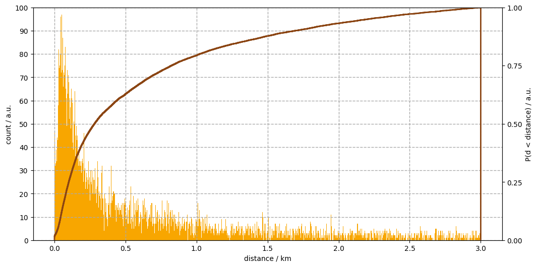
Figure 5. The occurences of the eighty most frequent pub names (golden ale bars). The cumulative distribution function of the entire set (stout line).

It is best left to the experts to ascertain what factors and processes formed the overall distribution. A few to mention

clustering effect i.e. small areas where pubs are concentrated
number of pubs in a settlement as a function of the settlement size
settlement size distribution
settlement spatial distribution

Shall we?