Python generator exercises. Part 5.: Sampling generator

The fifth post on generators sees guides the reader along the assembling of a sampler from the utilities defined in the previous posts. As a little treat, the resultant samples are analyses in the Bayesian framework.

Note

The raw notebook is has been made accessible here. The scripts are deposited in this folder.

Introduction

The first four sets of notes built various simple generators. The actions they performed assigned a role to them, according to which they were named. We proceed to combine them, with very little extra work, to make a sampler.

Coding style

It is apt and timely to remind ourselves, that these are exercises. The aim is to rely on basic (built-in) python features and aiming whilst using a constant memory whenever possible. Without recourse to third party libraries, such as numpy – especially in this post – would immensely reduce the coding effort and the complexity of their results.

Class sampler

Problem statement

We wish to create a batch of samples from different sources. A given number of elements must be included in each and every sample from each source.

Approach

The switcher function already yields samples from specified sources (or classes, if you wish). Therefore we need to instruct it to do two more tasks

1. select the required number of elements from each class
2. return these elements in batches

Pseudo-shuffling

As to the first point, there are many incorrect or poor solutions. Rather than pretending to be didactic, a correct algorithm is sketched straight away. It is based on sampling without replacement.

1. imagine a multiset as a vector
2. pick an element uniformly from the vector randomly and yield it
3. delete the element
4. go to 2. until no elements are left

The procedure above would require $O(N)$ storage where $N$ is the sample size. This can be changed to $O(k)$ where $k$ is the number of classes. It is achieved by only storing how many elements remain in each class.

Bookkeeping

Only the number of samples to be taken from each class, counts is needed to initialise the bookkeeping array.

def make_bookkeep(counts: Tuple[int]) -> List[int]:
    """
    Creates a bookeeping array which is used to track how many
    individuals can be taken from each class in order to
    create a full sample.
    """

    bookkeep = [0]
    for i, count in enumerate(counts):
        bookkeep.append(bookkeep[- 1] + count)

    return bookkeep

Shulling indices in a sample

1. arrange the class memberships in contiguous groups
   1. e.g.: ${A, A, A, B, B, B, B, C, C, C}$
2. Only record the running sum of the numbers of the identical elements
   1. e.g.: $\mathbb{N}^{k + 1} \ni \mathbf{a} \leftarrow (0, 3, 7, 10)$ from the array above
3. choose a random number from the range $i \sim \texttt{Uniform}([1, a_{k + 1}])$
   1. e.g.: $i \leftarrow 6$
4. find the first element of $\mathbf{a}$ which i) is smaller than $i$. The position of this element will be class index plus one
   1. e.g.: $c \leftarrow 2 = 3 - 1$
5. decrement $a_{j}, i \leq j$ by one if it is larger than $a_{j - 1}$
   1. e.g.: $\mathbf{a} \leftarrow (0, 3, 6, 9)$
6. Repeat from 2 until $\mathbf{a}$ consists of only zeros

sample_multiset_no_replacement is a generator of such a sequence of indices by realising the algorithm above.

def sample_multiset_no_replacement(bookkeep: Tuple[int]) -> Generator:
    """
    Generator of class indices in a sample.
    Each index appears at specified number
    of times in the sample and with equal probaibilty at any place.
    """

    # number of elements in all classes
    n = len(bookkeep)

    # until all elements are taken
    while bookkeep[-1] != 0:

        # choose an element index
        i_pos = np.random.randint( bookkeep[-1])

        # find the class range where the element index is
        for i_class, i_pos_class_max in enumerate(bookkeep):
            if i_pos < i_pos_class_max:
                yield i_class - 1
                break

        # decrement the class index ranges by one
        # 1) decrease the cardinality of the selected class ...
        # 2) ... and shift ranges to its right to the left
        for i in range(i_class, n):
            # only if there are elements left in the class
            if bookkeep[i] == bookkeep[i - 1]:
                continue
            bookkeep[i] -= 1

Yielding samples anew

In terms of our second concern, we only need to create an infinite generator of the sample_multiset_no_replacement generator. generate_sample_index_batches just does that whilst replenishing the bookkeeping array at every yield.

def generate_sample_index_batches(
        counts: Tuple[int]
    ) -> Generator:
    """
    Generator of batch class indices.
    Each index appears at specified number
    of times in the sample and with equal probaibilty at any place.
    """

    while True:
        bookkeep = make_bookkeep(counts)
        yield sample_multiset_no_replacement(bookkeep)

A few more lines are needed to combine the input streams of class indices (index_series) with the actual elements in the classes (iterators). The serialiser concatenates the class index batcher which is then combined with the underlying data sources in switcher. Finally, batches of the samples are formed by make_batcher.

def class_sampler(
        iterators: Tuple[Iterator],
        counts: Tuple[int]
    ) -> Generator:
    """
    Creates a generator of samples where each sample
    i) is a batch, ii) contains individuals from classes
    at a given number of times.
    """

    # first create a generator of class indices
    # each class appears the required number of times in each batch
    index_batches = generate_sample_index_batches(counts)

    # concatenate the batches so we can pass it to existing functions
    index_series = serialiser(index_batches)

    # contiguous samples
    gen_sample = switcher(iterators, index_series)

    # cut up to sample size batches
    samples = make_batcher(
        gen_sample, sum(counts), strict=False
    )

    return samples

Example

Elements of three classes are mixed in the fixed 3–1–6 ratio.

data_by_classes = tuple([
    repeat("a"), repeat("b"), repeat("c")
])

num_class_in_sample = tuple([3, 1, 6])

samples = class_sampler(data_by_classes, num_class_in_sample)

for i in range(3):
    sample = next(samples)
    print(list(sample))

['c', 'c', 'c', 'c', 'a', 'b', 'a', 'c', 'a', 'c']
['a', 'c', 'c', 'a', 'a', 'c', 'c', 'c', 'c', 'b']
['c', 'b', 'c', 'c', 'c', 'a', 'c', 'c', 'a', 'a']

Bayesian statistical testing

It is nothing but refreshing to abandon all these blocks of source code to dip in some statistics.

Goal

Let us playfully pretend the we are ignorant of the class frequencies in the sample beyond some rough estimates thereof. We will proceed to establish what class frequencies are likely given a set of samples.

Setup

The distribution of classes at a position is multinomial. A joint multinomial distribution describes the simultaneous probabilities of the class occurrences over all positions.

We focus on a given position in each batch of indices. A sample is the class values which have been realised at this position over all batches:

The random variable which represents the frequency of a class is denoted by $Q_{k}$. Its value has the symbol $q_{k}$. Likewise, the count of the elements which are of the $i$-th class is a random variable, $X_{i}$.

The observed count of this class is $x_{k}$. We wish to establish what the probabilities are of the different values of the unknown frequencies ($Q_{k}$) given the sample at hand:

in shorthand:

The probability of a realisation of the frequencies given the sample is conveniently expressed in Bayesian terms.:

After a handful manipulations, which are detailed in the Appendix, we arrive at the Bayesian probability density function of the frequencies conditioned on the observed sample. It is a Dirichlet distribution.

where $B(…)$ is the beta function.

Sample size

The smallest frequency will determine how many samples are needed. Let us then treat the ternary distribution as a binomial one for the sake of argument. There is an estimated class frequency, $\hat{q}$ of the least favoured class. All other outcomes will thus have a frequency of $1 - \hat{q}$.

We determine how many samples are required to have a sharp estimate ($\hat{q}$). By sharp it is meant that the maximum a posteriori estimate of the frequency is bracketed by two values of frequencies, $q_{l}, q_{u}$ where the total probability is concentrated:

There are a handful of issues:

1. we do not know $x_{1}$ or $x_{2}$ $\rightarrow$ we know that $\hat{q} \approx 0.1$ so that they can be estimated at a given $n$
2. even worse, our initial estimate of $q$ might be totally off. $\rightarrow$ this is where the power (pun intended) of the Bayesian analysis shows, by examining at the posterior distribution we can ascertain the goodness of our initial assumptions and update them accordingly
3. There are infinitely many such intervals. Even when $r$ is demanded to be the smallest possible of regions, there can be more than one depending on the shape of the cumulative distribution function $\rightarrow$ decide on the position of the interval in advance.

In short, we seek the number of samples where:

It turns out, about $4.1 \cdot 10^{3}$ samples are required.

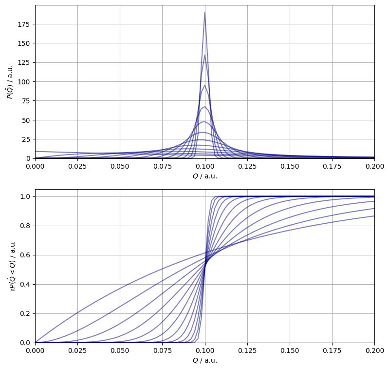
Figure 1. The pdf (top panel) and the cdf (bottom panel) of the estimated smallest frequency.

Figure 1. shows a posteriori binomial distribution functions. Each curve belong to a sample of size double that of the previous one. A surprising large sample is required to contain the estimate in a $\pm 0.05$ confidence band of the frequentist framework.

Hideous code time!

To further illustrate the previous observation a sequence of samples are generated of increasing size. The full Bayesian posterior are the calculated and plotted. As the keen reader will have noticed, we have relieved ourselves of the duty of writing generators. This is justified by keeping only a counter of classes in memory.

np.imag(counter) + 1,
    n_sample - np.real(counter) - np.imag(counter) + 1
]

Figure 2. The pdf of the first two class frequencies (shades between blue and white) the exact frequencies (black crosses), the maximum a priori estimates of the frequencies (orange crosses).

Whilst the maximum a priori estimates quickly converge to the exact values, their uncertainty decreases at a much lower rate, as evidenced by Figure 2.